Note
Go to the end to download the full example code
Cross-Frequency Coupling#
The spectrum tools in EMD can be used to explore cross-frequency interactions in oscillatory signals. The simplest approach is to look at how the phase, frequency or amplitude of a high-frequency signal interacts with the phase of a low frequency signal. This can be extended into 2 or 3 dimensions by exploring the relationship between low-frequency phase and the Hilbert-Huang Transform and Holospectrum. This tutorial shows some examples of these analyses with three signals with varying phase-amplitude coupling profiles.
Simulating a signal with amplitude modulations#
First of all, we import EMD alongside numpy and matplotlib. We will also use scipy’s ndimage module to smooth our results for visualisation later.
# sphinx_gallery_thumbnail_number = 8

import matplotlib.pyplot as plt
import numpy as np
import emd
Next, we create three simulated signal to analyse. Each signal will be composed of two oscillations - a low-frequency signal at 5Hz and a high-frequency signal at 37Hz. The three variants of this signal differ in how the amplitude of the high frequency signal varies with the phase of the low frequency signal. We vary the width of the high-frequency burst across the three signals.
seconds = 60
sample_rate = 200
t = np.linspace(0, seconds, seconds*sample_rate)

# First we create a slow 5Hz oscillation and a fast 37Hz oscillation
slow = np.sin(2*np.pi*5*t - np.pi/2)
fast = np.cos(2*np.pi*37*t)

# Next we create three different amplitude modulation signals for the fast
# oscillation. One sinusoidal, one wide modulation and one narrow modulation.
# These cases differ by the duration of the high frequency burst.

fast_am = 0.5*slow + 0.5
fast_am_narrow = fast_am**3
fast_am_wide = 1 - (0.5*-slow + 0.5)**3

# We create our signal by summing the oscillation and adding some noise
x = slow + fast * fast_am + np.random.randn(*t.shape) * .05
x_wide = slow + fast * fast_am_wide + np.random.randn(*t.shape) * .05
x_narrow = slow + fast * fast_am_narrow + np.random.randn(*t.shape) * .05
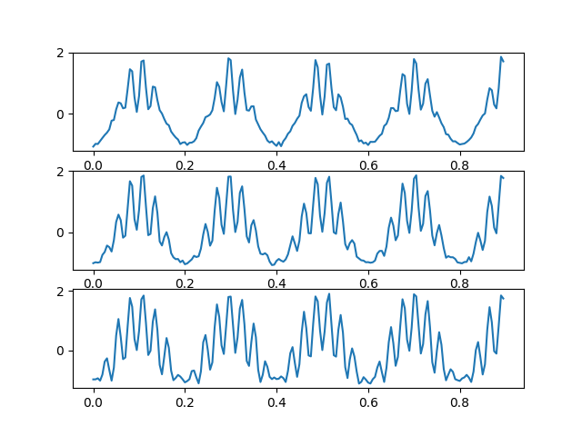
Let’s take a look at the three signals.
plt.figure()
plt.subplot(311)
plt.plot(t[:seconds*3], x_narrow[:seconds*3])
plt.subplot(312)
plt.plot(t[:seconds*3], x[:seconds*3])
plt.subplot(313)
plt.plot(t[:seconds*3], x_wide[:seconds*3])
[<matplotlib.lines.Line2D object at 0x7f4e455a3a50>]
The narrow amplitude modulated signal is plotted on the top, the sinusoidally modulated case in the middle and the wide amplitude modulation on the bottom. All three high-frequency signals peak at the same point in the low-frequency cycle.
Next we run a mask sift on these signals to create IMFs for each case before running the frequency transforms to get the instantaneous phase, frequency and phase.
# Define a mask sift config
config = emd.sift.get_config('mask_sift')
config['max_imfs'] = 7
config['mask_freqs'] = 50/sample_rate
config['mask_amp_mode'] = 'ratio_sig'
config['imf_opts/sd_thresh'] = 0.05
config['extrema_opts/method'] = 'rilling'

imf = emd.sift.mask_sift(x, **config)
IP, IF, IA = emd.spectra.frequency_transform(imf, sample_rate, 'hilbert')

imf_wide = emd.sift.mask_sift(x_wide, **config)
IP_wide, IF_wide, IA_wide = emd.spectra.frequency_transform(imf_wide, sample_rate, 'hilbert')

imf_narrow = emd.sift.mask_sift(x_narrow, **config)
IP_narrow, IF_narrow, IA_narrow = emd.spectra.frequency_transform(imf_narrow, sample_rate, 'hilbert')
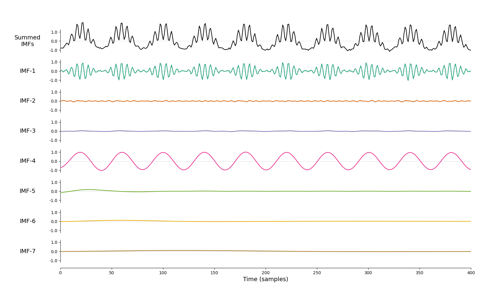
We plot up the IMFs for the sinusoidally modulated case and see that the fast signal is isolated into the first IMF and the low-frequency signal is in the fourth. The rest of the IMFs largely contain noise
emd.plotting.plot_imfs(imf[:sample_rate*2, :])
<Axes: xlabel='Time (samples)'>
1D Phase-amplitude coupling with instantaneous amplitude#
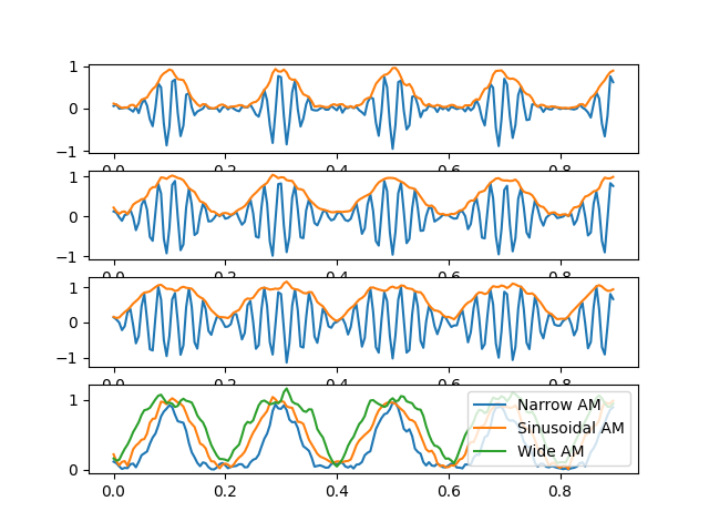
Let’s zoom in on the fast signals containing the simulated amplitude modulations. Here, we plot the first IMF for each of the three signals with different modulation widths.
plt.figure()
plt.subplot(411)
plt.plot(t[:seconds*3], imf_narrow[:seconds*3, 0])
plt.plot(t[:seconds*3], IA_narrow[:seconds*3, 0])
plt.subplot(412)
plt.plot(t[:seconds*3], imf[:seconds*3, 0])
plt.plot(t[:seconds*3], IA[:seconds*3, 0])
plt.subplot(413)
plt.plot(t[:seconds*3], imf_wide[:seconds*3, 0])
plt.plot(t[:seconds*3], IA_wide[:seconds*3, 0])
plt.subplot(414)
plt.plot(t[:seconds*3], IA_narrow[:seconds*3, 0])
plt.plot(t[:seconds*3], IA[:seconds*3, 0])
plt.plot(t[:seconds*3], IA_wide[:seconds*3, 0])
plt.legend(['Narrow AM', 'Sinusoidal AM', 'Wide AM'])
<matplotlib.legend.Legend object at 0x7f4e54401550>
The narrow modulation is on top-row, the sinusoidal modulation in the second and the wide modulation is in the third. All three amplitude modulations on top of each other in the bottom row. By eye, the different modulation widths are clear but it is perhaps less obvious how we can quantify this effect.
One simple approach is to explore how the instantaneous amplitude of each
case varies with the phase of the low-frequency signal component. We can
compute this with emd.cycles.bin_by_phase. The inputs take a phase signal
which is segmented into a set of time-bins in which the second input is
averaged. (A very similar alternative analysis could be run using
emd.cycles.phase_align).
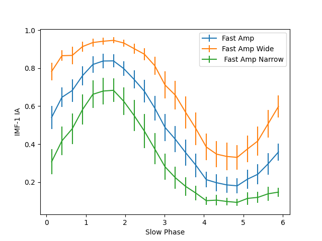
We compute the average high-frequency IA as a function of low-frequency phase for each of our three examples and plot the result:
ia_by_phase, ia_by_phase_var, phase_bins = emd.cycles.bin_by_phase(IP[:, 4], IA[:, 0], nbins=24)
ia_by_phase_wide, ia_by_phase_wide_var, _ = emd.cycles.bin_by_phase(IP[:, 4], IA_wide[:, 0], nbins=24)
ia_by_phase_narrow, ia_by_phase_narrow_var, _ = emd.cycles.bin_by_phase(IP[:, 4], IA_narrow[:, 0], nbins=24)

plt.figure()
plt.errorbar(phase_bins, ia_by_phase, yerr=ia_by_phase_var)
plt.errorbar(phase_bins, ia_by_phase_wide, yerr=ia_by_phase_wide_var)
plt.errorbar(phase_bins, ia_by_phase_narrow, yerr=ia_by_phase_narrow_var)
plt.legend(['Fast Amp', 'Fast Amp Wide', ' Fast Amp Narrow'])
plt.xlabel('Slow Phase')
plt.ylabel('IMF-1 IA')
Text(42.722222222222214, 0.5, 'IMF-1 IA')
Now, we see the three amplitude modulation profiles directly linked to theta phase - there is a clear peak in high-frequency amplitude at one point in theta phase confirming the presence of phase-amplitude coupling in this signal. We can also see the different in modulation width in the three signals.
2D Phase-amplitude coupling with the HHT#
We can run a two-dimensional equivalent to the above analysis by exploring how a whole Hilbert-Huang transform varies across low-frequency phase. This gives us a bit more information than our first analysis. Specifically we can also see which frequency the amplitude modulated signal is peaking at.
The first step is to compute the Hilbert-Huang Transform (HHT) for our three signals.
freq_edges, freq_centres = emd.spectra.define_hist_bins(10, 75, 75, 'log')

f, hht = emd.spectra.hilberthuang(IF, IA, freq_edges, mode='amplitude', sum_time=False)
f, hht_wide = emd.spectra.hilberthuang(IF_wide, IA_wide, freq_edges, mode='amplitude', sum_time=False)
f, hht_narrow = emd.spectra.hilberthuang(IF_narrow, IA_narrow, freq_edges, mode='amplitude', sum_time=False)
A quick summary figure shows us the HHT representation of our amplitude modulated signals. The recurring high-frequency bursts are visible in all three cases with the duration of each burst differing between the narrow, sinusoidal and widde cases.
plt.figure()
plt.subplot(411)
plt.plot(t[:seconds*3], x[:seconds*3])
plt.subplot(412)
plt.pcolormesh(t[:seconds*3], f, hht_narrow[:, :seconds*3], cmap='hot_r', shading='auto')
plt.subplot(413)
plt.pcolormesh(t[:seconds*3], f, hht[:, :seconds*3], cmap='hot_r', shading='auto')
plt.subplot(414)
plt.pcolormesh(t[:seconds*3], f, hht_wide[:, :seconds*3], cmap='hot_r', shading='auto')
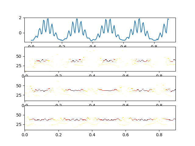
<matplotlib.collections.QuadMesh object at 0x7f4e446abdd0>
We can use emd.cycles.bin_by_phase to explore how high dimensional
signals vary with a phase time-course - as long as the first dimension of the
signal to be averaged matches the length of the phase signal. Here, we bin
the HHT by low-frequency phase for each of our three signals.
hht_by_phase, _, phase_centres = emd.cycles.bin_by_phase(IP[:, 4], hht.T)
hht_by_phase_wide, _, _ = emd.cycles.bin_by_phase(IP[:, 4], hht_wide.T)
hht_by_phase_narrow, _, _ = emd.cycles.bin_by_phase(IP[:, 4], hht_narrow.T)
Let’s make a quick summary figure of the phase-resolved HHTs.
plt.figure()
plt.subplot(131)
plt.pcolormesh(phase_centres, freq_centres, hht_by_phase_narrow.T, vmax=0.25, cmap='hot_r', shading='auto')
plt.xlabel('Phase (rads')
plt.ylabel('Frequency (Hz)')
plt.title('Narrow AM')
plt.subplot(132)
plt.pcolormesh(phase_centres, freq_centres, hht_by_phase.T, vmax=0.25, cmap='hot_r', shading='auto')
plt.xlabel('Phase (rads')
plt.title('Sinusoidal AM')
plt.subplot(133)
plt.pcolormesh(phase_centres, freq_centres, hht_by_phase_wide.T, vmax=0.25, cmap='hot_r', shading='auto')
plt.xlabel('Phase (rads')
plt.title('Wide AM')
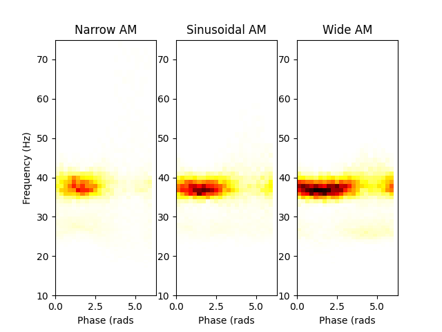
Text(0.5, 1.0, 'Wide AM')
We can see that all three cases peak around the same point in phase (around pi/2) at at the same frequency (37Hz) but clearly differ in their modulation width. Though this is visible here, we still don’t directly quantify this feature with the Hilbert-Huang Transform.
We can quantify this difference by looking at the frequency content of the high-frequency signal amplitude envelopes. It appears like the signal with wide modulation has a lower frequency amplitude modulation How can we measure this?
Quantifying the frequency of amplitude modulations#
The Holospectrum provides a method for direct quantification of the frequency and timing of amplitude modulations in oscillatory signal. The concept and method for Holospectrum estimation are covered in detail in the previous tutorial - here we will only cover its application in cross-frequency coupling.
First, we compute the second-layer sift of our amplitude modulated signals. We apply a mask-sift at the second level to the instantaneous amplitude of our high frequency signals. The frequency transform of the resulting second-layer IMFs is then computed using the Hilbert transform.
# Reduce the mask frequencies for the second layer sift - otherwise we use the
# same config as the first layer.
config['mask_freqs'] = [10/sample_rate/ii for ii in range(1, 10)]


imf2 = emd.sift.mask_sift_second_layer(IA[:, 0], config['mask_freqs'], sift_args=config)
IP2, IF2, IA2 = emd.spectra.frequency_transform(imf2, sample_rate, 'hilbert')

imf2_wide = emd.sift.mask_sift_second_layer(IA_wide[:, 0], config['mask_freqs'], sift_args=config)
IP2_wide, IF2_wide, IA2_wide = emd.spectra.frequency_transform(imf2_wide, sample_rate, 'hilbert')

imf2_narrow = emd.sift.mask_sift_second_layer(IA_narrow[:, 0], config['mask_freqs'], sift_args=config)
IP2_narrow, IF2_narrow, IA2_narrow = emd.spectra.frequency_transform(imf2_narrow, sample_rate, 'hilbert')
Next we compute the Holospectrum itself. We define a two sets of frequency
bins for the first layer oscillations and second layer amplitude modulations
before computing the Holospectrum using emd.spectra.holospectrum.
freq_edges, freq_centres = emd.spectra.define_hist_bins(1, 75, 75, 'log')
freq_edges_low, freq_centres_low = emd.spectra.define_hist_bins(2, 10, 20, 'linear')

fcarrier, fam, holo = emd.spectra.holospectrum(IF[:, 0, None], IF2, IA2, freq_edges, freq_edges_low)
fcarrier, fam, holo_narrow = emd.spectra.holospectrum(IF_narrow[:, 0, None], IF2_narrow, IA2_narrow, freq_edges, freq_edges_low)
fcarrier, fam, holo_wide = emd.spectra.holospectrum(IF_wide[:, 0, None], IF2_wide, IA2_wide, freq_edges, freq_edges_low)

# Holo is [second-layer frequencies x first-layer frequencies]
print(holo.shape)
(75, 20)
The output holospectrum is a 2d matrix of first-layer frequencies by second-layer frequencies (we sum across time dimension by default). We next make a summary plot with this 2d Holospectrum for each case in the top row and the average holospectrum across first-layer frequencies (ie expressing the energy in signals with given amplitude modulation frequencies across all first-layer frequencies.)
plt.figure()
plt.subplot(231)
plt.pcolormesh(freq_centres_low, freq_centres, holo_narrow, cmap='hot_r', shading='auto')
plt.ylabel('Frequency (Hz)')
plt.xticks(np.arange(3, 10, 2))
plt.title('Narrow AM')
plt.subplot(234)
plt.plot(freq_centres_low, holo_narrow[62, :])
plt.xlabel('AM Frequency (Hz)')
plt.xticks(np.arange(3, 10, 2))
plt.ylabel('Amplitude')

plt.subplot(232)
plt.pcolormesh(freq_centres_low, freq_centres, holo, cmap='hot_r', shading='auto')
plt.xticks(np.arange(3, 10, 2))
plt.title('Sinusoidal AM')
plt.subplot(235)
plt.plot(freq_centres_low, holo[62, :])
plt.xticks(np.arange(3, 10, 2))
plt.xlabel('AM Frequency (Hz)')

plt.subplot(233)
plt.pcolormesh(freq_centres_low, freq_centres, holo_wide, cmap='hot_r', shading='auto')
plt.xticks(np.arange(3, 10, 2))
plt.title('Wide AM')
plt.subplot(236)
plt.plot(freq_centres_low, holo_wide[62, :])
plt.xticks(np.arange(3, 10, 2))
plt.xlabel('AM Frequency (Hz)')
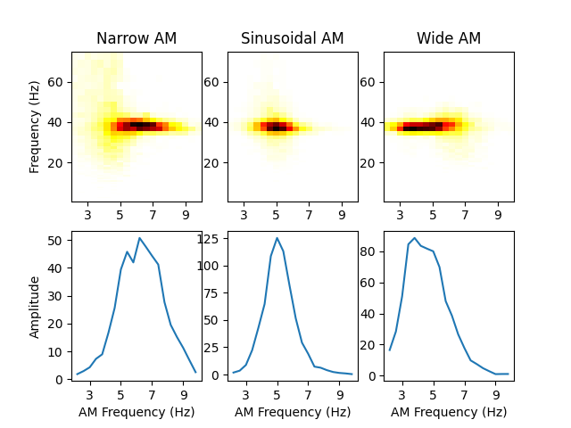
Text(0.5, 23.52222222222222, 'AM Frequency (Hz)')
The holospectra on the top row show the distribution of energy across frequency and amplitude modulation frequency within each signal. The bottom row sums the holospectra across the y-axis to summarise just the distribution of energy across apmlitude modulation frequencies.
The sinusoidal signal has a clear peak with a frequency of 37Hz with amplitude modulations of 5Hz - exactly as we would expect from this simulation. The other signals have a similar peak but slightly skewed to higher or lower amplitude modulation frequencies. The signal with narrow modulation has higher amplitude modulation frequencies - reflecting the faster/sharper amplitude modulation profile of the signal. In contrast, the signal with wide amplitude modulations skews towards slower amplitude modulations - reflectings its slower, flatter amplitude modulation profile.
The holospectrum provides a convenient summary of the amplitude modulations in a signal, but doesn’t explicitly link them to the phase of a lower frequency signal. To complete a full cross-frequency coupling analysis with the Holospectrum we need to show not only that our high frequency signal has amplitude modulations but that those amplitude modulations are specifically linked to a n observed low-frequency signal.
3D phase-amplitude coupling with the Holospectrum#
We can link the Holospectrum to low frequency phase in exactly the same way
as we analysed the instantaneous amplitude and Hilbert-Huang Transforms.
First, we have to recompute the holospectra whilst preserving the time
dimension in the output. By default, the holospectrum is summed over time
before being returned - we can ask for the full 3D holospectrum to be
returned by setting squash_time=False in the emd.spectra.holospectrum
call.
# Define a new set of second-layer frequencies - slightly wider than the last one.
freq_edges_low, freq_centres_low = emd.spectra.define_hist_bins(.5, 15, 32, 'linear')

fcarrier, fam, holot = emd.spectra.holospectrum(IF[:, 0, None], IF2, IA2,
                                 freq_edges, freq_edges_low, sum_time=False)
fcarrier, fam, holot_wide = emd.spectra.holospectrum(IF_wide[:, 0, None], IF2_wide, IA2_wide,
                                      freq_edges, freq_edges_low, sum_time=False)
fcarrier, fam, holot_narrow = emd.spectra.holospectrum(IF_narrow[:, 0, None], IF2_narrow, IA2_narrow,
                                        freq_edges, freq_edges_low, sum_time=False)


# holot is [second-layer frequencies x first-layer frequencies x time samples]
print(holot.shape)
(75, 32, 12000)
Now that we have a time-varying holospectrum estimate - we can compute its
average in different low-frequency bins by using emd.cycles.bin_by_phase
as for our previous analyses.
holo_by_phase, _, phase_bins = emd.cycles.bin_by_phase(IP[:, 4], np.swapaxes(holot, 0, 2))
holo_by_phase_wide, _, _ = emd.cycles.bin_by_phase(IP[:, 4], np.swapaxes(holot_wide, 0, 2))
holo_by_phase_narrow, _, _ = emd.cycles.bin_by_phase(IP[:, 4], np.swapaxes(holot_narrow, 0, 2))

# holo_by_phase is [phase bins x second-layer frequencies x first-layer frequencies]
print(holo_by_phase.shape)
(24, 32, 75)
holo_by_phase now contains a summary of the energy in each signal
separated by first-layer frequencies, second layer-frequencies and by the
phase of our low frequency signal. If the amplitude modulations we observed
in our signals are explicitly linked to the 5Hz phase - we should be able to
see it here.
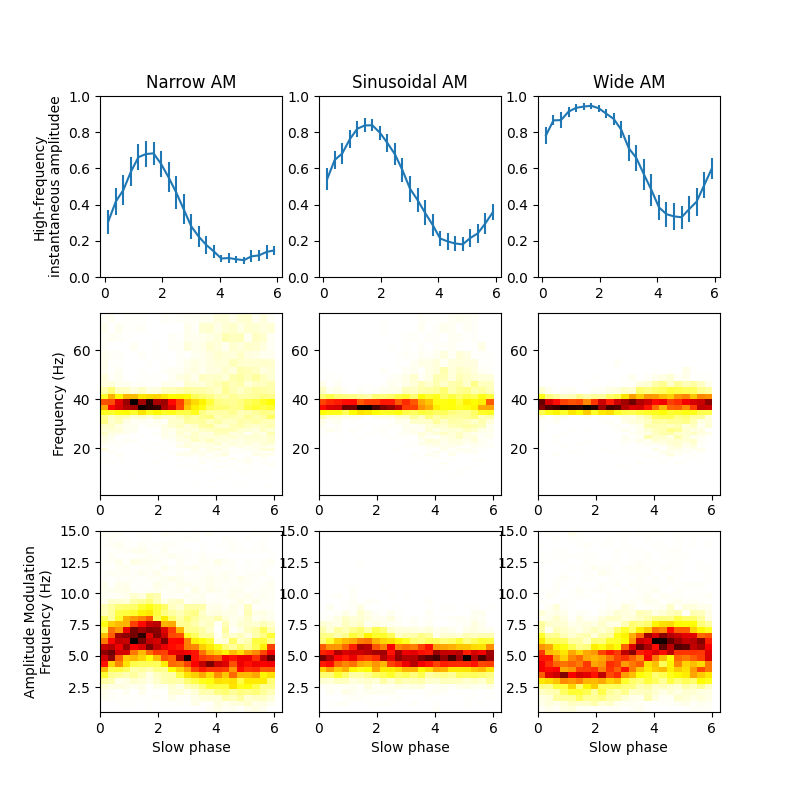
We can summarise holo_by_phase a few ways. To start we we plot the
high-frequency instantaneous amplitude on the top-row for reference. The
second row contains the first-layer frequencies in the Holospectrum as a
function of 5Hz phase, finally the third row contains the second-layer
amplitude modulation frequencies across 5Hz phase.
plt.figure(figsize=(8, 8))
plt.subplot(331)
plt.errorbar(phase_bins, ia_by_phase_narrow, yerr=ia_by_phase_narrow_var)
plt.ylim(0, 1)
plt.ylabel('High-frequency\ninstantaneous amplitudee')
plt.title('Narrow AM')
plt.subplot(332)
plt.errorbar(phase_bins, ia_by_phase, yerr=ia_by_phase_var)
plt.ylim(0, 1)
plt.title('Sinusoidal AM')
plt.subplot(333)
plt.errorbar(phase_bins, ia_by_phase_wide, yerr=ia_by_phase_wide_var)
plt.ylim(0, 1)
plt.title('Wide AM')

plt.subplot(334)
plt.pcolormesh(phase_centres, freq_centres, holo_by_phase_narrow.sum(axis=1).T,  cmap='hot_r', shading='auto')
plt.ylabel('Frequency (Hz)')
plt.subplot(335)
plt.pcolormesh(phase_centres, freq_centres, holo_by_phase.sum(axis=1).T, cmap='hot_r', shading='auto')
plt.subplot(336)
plt.pcolormesh(phase_centres, freq_centres, holo_by_phase_wide.sum(axis=1).T, cmap='hot_r', shading='auto')

plt.subplot(337)
plt.pcolormesh(phase_centres, freq_centres_low, holo_by_phase_narrow.sum(axis=2).T, cmap='hot_r', shading='auto')
plt.ylabel('Amplitude Modulation\nFrequency (Hz)')
plt.xlabel('Slow phase')
plt.subplot(338)
plt.pcolormesh(phase_centres, freq_centres_low, holo_by_phase.sum(axis=2).T, cmap='hot_r', shading='auto')
plt.xlabel('Slow phase')
plt.subplot(339)
plt.pcolormesh(phase_centres, freq_centres_low, holo_by_phase_wide.sum(axis=2).T, cmap='hot_r', shading='auto')
plt.xlabel('Slow phase')
Text(0.5, 58.7222222222222, 'Slow phase')
The second row here is very similar to the HHT-by-phase plot in our previous section and confirms that there is a peak in 37Hz power around pi/2 in the low-frequency phase. Again, the width of the modulation is visible as stretching of the peak in the x-axis.
The third row gives us some new information about how amplitude modulation frequency of the 37Hz frequency signal changes across the phase of the 5Hz signal. This is a flat profile at 5Hz for the sinsoidal signal but changes for the narrow and wide case. Critically the narrow amplitude modulation has an increase in amplitude modulation frequency around pi/2 - the point in the low-frequency signal where the high-frequency signal peaks. In contrast, the wide modulation signal has a lower amplitude modulation frequency at the same point. This reflects the fast-sharp peak in the narrow modualtion and the flat peak in the wide modulation.
All three signals are clearly linked to the low-frequency phase. Interestingly, the holospectrum is able to quantify the non-linear differences in amplitude modulation frequency driven by the diferences in modulation width.
Further Reading & References#
Huang, N. E., Shen, Z., Long, S. R., Wu, M. C., Shih, H. H., Zheng, Q., … Liu, H. H. (1998). The empirical mode decomposition and the Hilbert spectrum for nonlinear and non-stationary time series analysis. Proceedings of the Royal Society of London. Series A: Mathematical, Physical and Engineering Sciences, 454(1971), 903–995. https://doi.org/10.1098/rspa.1998.0193
Huang, N. E., Hu, K., Yang, A. C. C., Chang, H.-C., Jia, D., Liang, W.-K., … Wu, Z. (2016). On Holo-Hilbert spectral analysis: a full informational spectral representation for nonlinear and non-stationary data. Philosophical Transactions of the Royal Society A: Mathematical, Physical and Engineering Sciences, 374(2065), 20150206. https://doi.org/10.1098/rsta.2015.0206
Total running time of the script: (0 minutes 5.129 seconds)