Note
Go to the end to download the full example code
The ‘Cycles’ class#
EMD provides a Cycles class to help with more complex cycle comparisons. This class is based on the emd.cycles.get_cycle_vector and emd.cycles.get_cycle_stat functions we used in the previous tutorial, but it does some additional work for you. For example, the Cycles class is a good way to compute and store many different stats from the same cycles and for dynamically working with different subsets of cycles based on user specified conditions. Lets take a closer look…
Getting started#
Firstly we will import emd and simulate a signal.
import emd
import numpy as np
import matplotlib.pyplot as plt
# Define and simulate a simple signal
peak_freq = 15
sample_rate = 256
seconds = 10
noise_std = .4
x = emd.simulate.ar_oscillator(peak_freq, sample_rate, seconds,
noise_std=noise_std, random_seed=42, r=.96)[:, 0]
t = np.linspace(0, seconds, seconds*sample_rate)
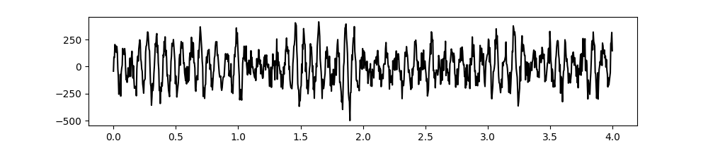
# Plot the first 5 seconds of data
plt.figure(figsize=(10, 2))
plt.plot(t[:sample_rate*4], x[:sample_rate*4], 'k')
# sphinx_gallery_thumbnail_number = 4
[<matplotlib.lines.Line2D object at 0x7f4e4439a3d0>]
We next run a mask sift with the default parameters to isolate the 15Hz oscillation. There is only one clear oscillatory signal in this simulation. This is extracted in IMF-2 whilst the remaining IMFs contain low-amplitude noise.
# Run a mask sift
imf = emd.sift.mask_sift(x, max_imfs=5)

# Computee frequenecy transforms
IP, IF, IA = emd.spectra.frequency_transform(imf, sample_rate, 'hilbert')
The Cycles class#
We next initialise the ‘Cycles’ class with the instantaneous phase of the second IMF.
C = emd.cycles.Cycles(IP[:, 2])
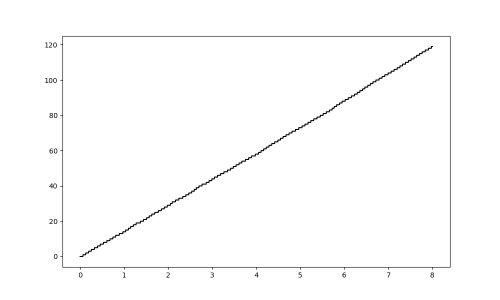
This calls emd.cycles.get_cycle_vect on the phase time course to identify individual cycles and then stores a load of relevant information which we can use later. The cycle vector is stored in the class instance as cycle_vect. Here we plot the cycle vector for the first four seconds of our signal.
plt.figure(figsize=(10, 6))
plt.plot(t[:sample_rate*8], C.cycle_vect[:sample_rate*8], 'k')
[<matplotlib.lines.Line2D object at 0x7f4e3ffe3190>]
The Cycles class has an attached function to help identify when specific
cycles occurred in a dataset. The C.get_inds_of_cycle function finds and
returns the samples in which the Nth cycle occurred. Here, we run this find
and plot three cycles from our simulation. The cycle in the original
time-series is plotted in grey and the cycle from the second IMF is in
colour.
cycles_to_plot = [5, 23, 43, 58, 99]
plt.figure()
for ii in range(len(cycles_to_plot)):
    inds = C.get_inds_of_cycle(cycles_to_plot[ii])
    xinds = np.arange(len(inds)) + 30*ii
    plt.plot(xinds, x[inds], color=[0.8, 0.8, 0.8])
    plt.plot(xinds, imf[inds, 2])
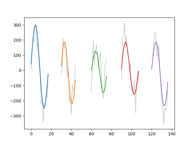
These cycles contain one complete period of an oscillation and form the basis for a lot of the computations in this tutorial. However there are a couple of shortcomings with this standard cycle. For example, we may want to separately analyse the ascending and descending edges of the oscillation, whilst the descending edge is continuous - the cycles above contain two halves of two separate ascending edges at the start and end of the cycle.
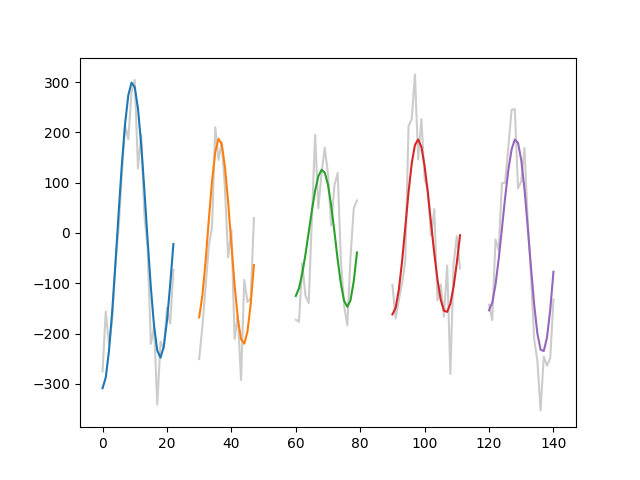
We could adjust the phase to make our cycle identification start at the peak to ensure the ascending edge is continuous, but this will just split another part of the cycle… One way around this is to consider an ‘augmented’ cycle which contains a whole standard cycle plus the last quadrant of the proceeding cycle. These five quarters of a cycle mean that all sections of the cycle are continuously represented, though it does meaen that some parts of the data may be present in more than one cycle.
We can work with augmented cycles by specifying mode='augmented' when
finding our cycle indices.
cycles_to_plot = [5, 23, 43, 58, 99]
plt.figure()
for ii in range(len(cycles_to_plot)):
    inds = C.get_inds_of_cycle(cycles_to_plot[ii], mode='augmented')
    xinds = np.arange(len(inds)) + 30*ii
    plt.plot(xinds, x[inds], color=[0.8, 0.8, 0.8])
    plt.plot(xinds, imf[inds, 2])
The cycles class can be used as an input to several other emd.cycles
functions to specify which cycles a particular computation should run across.
For example, here we compute the control points across from IMF-3 for each of our cycles.
ctrl = emd.cycles.get_control_points(imf[:, 2], C)
…and here we run phase-alignment.
pa = emd.cycles.phase_align(IP[:, 2], IF[:, 2], C)
/home/docs/checkouts/readthedocs.org/user_builds/emd/envs/latest/lib/python3.11/site-packages/scipy/interpolate/_interpolate.py:710: RuntimeWarning: divide by zero encountered in divide
  slope = (y_hi - y_lo) / (x_hi - x_lo)[:, None]
Computing cycle metrics#
We can loop through our cycles using the C.get_inds_of_cycle function to
identify a each cycle in turn. Here we run a loop to compute the maximum
amplitude of each cycle.
amps = np.zeros((C.ncycles,))
for ii in range(C.ncycles):
    inds = C.get_inds_of_cycle(ii)
    amps[ii] = np.max(IA[inds, 2])

print(amps)
[192.98594916 182.01754737 175.17040462 226.81503852 315.47911405
 313.95538144 234.47123024 238.13870334 177.82116937 256.62639472
 282.33371361 194.49536091 166.53168973 203.33782935 249.90525556
 204.88512803  69.54630875  82.52259582  82.94456599 126.91142784
 287.15379557 362.34201487 305.94413982 232.57942391 247.58394774
 168.84921598 359.36340717 405.56936258 300.136833   103.59726779
  55.92943445 111.0206236  116.84485754 153.70027248 156.71488824
 152.05436012 191.17808685 196.44364772  96.67404025 120.73336374
 120.57282357 106.20217088 128.44143838 164.63520255 243.73286264
 269.28189281 238.00670001 357.29404122 204.75434239  99.62869461
 143.49815985 185.42128791 193.22295992 178.52162508 126.38460715
 212.8333045  226.15932918 182.30892193 188.99604047 150.1371452
 137.00542555 121.63029869 159.61978656 215.41221478 240.36402985
 233.20696618 257.31510744 359.89979945 393.29438512 399.18796263
 293.37945587 402.22144702 391.48098615 432.98330155 429.96267513
 411.07068504 214.42333167 216.60074001 209.63650352 148.35286002
 268.01049566 334.60884625 325.45998299 321.17685882 128.56724027
 224.39978894 274.99449291 135.93143953 269.87368539 271.00306621
 233.08245956 261.19813423 243.23101988 169.25691486 125.91549686
  68.00383253  80.13349249 149.66364429 168.03964068 277.24824556
 352.60058695 375.01613643 364.25407461 181.06102301 325.73935455
 356.62423902 358.12461482 159.2589322  136.13954475 132.39063079
 198.50535673 228.93445339 187.43823377 214.61116591 247.52773184
 293.15011208 321.17912616 193.42905247 124.40162347  92.16732834
 207.46477627 411.25756332 412.30307304 355.93118476 249.96502386
 265.38238326 265.15890418 177.11911223 119.19597405 100.70339757
 127.20378459 113.33604931  48.11563467 104.99038027 263.79851284
 281.56940974 223.6829564  241.12859203 310.08490902 314.53899405
 339.33123531 306.07348852 215.72305388 211.64959472 178.32945638
 101.99703257  92.77461961 185.85625019 197.45277427 180.38022941]
The Cycles class has a handy method to help automate this process. Simply
specify a metric name, some values to compute a per-cycle metric on and a
function and C.compute_cycle_metric will loop across all cycles and store
the result for you.
C.compute_cycle_metric('max_amp', IA[:, 2], func=np.max)
This is always computed for every cycle in the dataset, we can include or exclude cycles based on different conditions later.
For another example we compute the length of each cycle in samples.
# Compute the length of each cycle
C.compute_cycle_metric('duration', IA[:, 2], len)
Cycle metrics can also be computed on the augmented cycles. Lets compute the standard deviation of amplitude values for each augmented cycle.
C.compute_cycle_metric('ampSD', IA[:, 2], np.std, mode='augmented')
We have now computed four different metrics across our cycles.
print(C)
<class 'emd.cycles.Cycles'> (150 cycles 4 metrics)
These values are now stored in the metrics dictionary along with the good cycle values.
print(C.metrics.keys())

print(C.metrics['is_good'])
print(C.metrics['max_amp'])
print(C.metrics['duration'])
dict_keys(['is_good', 'max_amp', 'duration', 'ampSD'])
[0 1 1 0 1 1 0 1 0 0 1 0 1 0 0 1 0 1 0 0 1 1 0 0 0 1 1 0 0 0 0 0 1 1 0 1 1
 0 0 0 0 1 0 1 1 1 1 1 1 0 1 0 1 1 1 1 0 0 1 0 1 0 0 0 0 1 0 0 1 1 0 0 1 1
 0 0 1 1 0 0 1 1 1 0 1 0 1 0 0 0 0 1 0 1 1 0 1 0 0 0 0 1 0 0 1 0 1 1 0 0 0
 0 1 0 0 1 0 0 1 1 0 1 0 1 1 0 1 0 0 1 1 0 0 1 0 0 1 0 0 1 1 1 0 0 1 1 0 0
 1 0]
[192.98594916 182.01754737 175.17040462 226.81503852 315.47911405
 313.95538144 234.47123024 238.13870334 177.82116937 256.62639472
 282.33371361 194.49536091 166.53168973 203.33782935 249.90525556
 204.88512803  69.54630875  82.52259582  82.94456599 126.91142784
 287.15379557 362.34201487 305.94413982 232.57942391 247.58394774
 168.84921598 359.36340717 405.56936258 300.136833   103.59726779
  55.92943445 111.0206236  116.84485754 153.70027248 156.71488824
 152.05436012 191.17808685 196.44364772  96.67404025 120.73336374
 120.57282357 106.20217088 128.44143838 164.63520255 243.73286264
 269.28189281 238.00670001 357.29404122 204.75434239  99.62869461
 143.49815985 185.42128791 193.22295992 178.52162508 126.38460715
 212.8333045  226.15932918 182.30892193 188.99604047 150.1371452
 137.00542555 121.63029869 159.61978656 215.41221478 240.36402985
 233.20696618 257.31510744 359.89979945 393.29438512 399.18796263
 293.37945587 402.22144702 391.48098615 432.98330155 429.96267513
 411.07068504 214.42333167 216.60074001 209.63650352 148.35286002
 268.01049566 334.60884625 325.45998299 321.17685882 128.56724027
 224.39978894 274.99449291 135.93143953 269.87368539 271.00306621
 233.08245956 261.19813423 243.23101988 169.25691486 125.91549686
  68.00383253  80.13349249 149.66364429 168.03964068 277.24824556
 352.60058695 375.01613643 364.25407461 181.06102301 325.73935455
 356.62423902 358.12461482 159.2589322  136.13954475 132.39063079
 198.50535673 228.93445339 187.43823377 214.61116591 247.52773184
 293.15011208 321.17912616 193.42905247 124.40162347  92.16732834
 207.46477627 411.25756332 412.30307304 355.93118476 249.96502386
 265.38238326 265.15890418 177.11911223 119.19597405 100.70339757
 127.20378459 113.33604931  48.11563467 104.99038027 263.79851284
 281.56940974 223.6829564  241.12859203 310.08490902 314.53899405
 339.33123531 306.07348852 215.72305388 211.64959472 178.32945638
 101.99703257  92.77461961 185.85625019 197.45277427 183.85172864]
[17 16 17 16 18 18 16 18 20 18 17 16 21 21 16 16 13 16 16 25 18 18 15 15
 17 21 18 17 17 18 11 19 19 23 18 17 17 15 12 15 18 24 17 16 15 18 18 19
 21 18 16 16 17 16 21 19 17 22 18 15 15 15 16 16 17 19 15 15 17 18 17 20
 19 19 17 18 16 17 19 19 17 18 18 16 12 14 17 15 18 18 18 18 16 15 16 13
 17 15 15 17 19 17 16 19 18 17 18 16 15 17 17 16 17 15 16 16 18 18 18 14
 14 18 16 18 18 16 18 17 15 15 17 18 12 18 17 16 16 14 18 17 17 18 17 18
 19 19 14 16 19 19]
These values can be accessed and used for further analyses as needed. The metrics can be copied into a pandas dataframe for further analysis if convenient.
df = C.get_metric_dataframe()
print(df)
     is_good     max_amp  duration      ampSD
0          0  192.985949        17        NaN
1          1  182.017547        16  30.297019
2          1  175.170405        17  22.371911
3          0  226.815039        16  20.954405
4          1  315.479114        18  34.657937
..       ...         ...       ...        ...
145        1  101.997033        19   8.031846
146        0   92.774620        14   2.500551
147        0  185.856250        16  32.345212
148        1  197.452774        19   7.232020
149        0  183.851729        19  12.624663

[150 rows x 4 columns]
We can extract a cycle vector for only the good cycles using the get_matching_cycles method attached to the Cycles class. This function takes a list of one or more conditions and returns a booleaen vector indicating which cycles match the conditions. These conditions specify the name of a cycle metric, a standard comparator (such as ==, > or <) and a comparison value.
Here, we will identify which cycles are passing our good cycle checks.
good_cycles = C.get_matching_cycles(['is_good==1'])
print(good_cycles)
[False  True  True False  True  True False  True False False  True False
  True False False  True False  True False False  True  True False False
 False  True  True False False False False False  True  True False  True
  True False False False False  True False  True  True  True  True  True
  True False  True False  True  True  True  True False False  True False
  True False False False False  True False False  True  True False False
  True  True False False  True  True False False  True  True  True False
  True False  True False False False False  True False  True  True False
  True False False False False  True False False  True False  True  True
 False False False False  True False False  True False False  True  True
 False  True False  True  True False  True False False  True  True False
 False  True False False  True False False  True  True  True False False
  True  True False False  True False]
This returns a boolean array indicating which cycles meet the specified conditions.
print('{0} matching cycles found'.format(np.sum(good_cycles)))
69 matching cycles found
and which cycles are failing…
bad_cycles = C.get_matching_cycles(['is_good==0'])
print('{0} matching cycles found'.format(np.sum(bad_cycles)))
print(bad_cycles)
81 matching cycles found
[ True False False  True False False  True False  True  True False  True
 False  True  True False  True False  True  True False False  True  True
  True False False  True  True  True  True  True False False  True False
 False  True  True  True  True False  True False False False False False
 False  True False  True False False False False  True  True False  True
 False  True  True  True  True False  True  True False False  True  True
 False False  True  True False False  True  True False False False  True
 False  True False  True  True  True  True False  True False False  True
 False  True  True  True  True False  True  True False  True False False
  True  True  True  True False  True  True False  True  True False False
  True False  True False False  True False  True  True False False  True
  True False  True  True False  True  True False False False  True  True
 False False  True  True False  True]
Several conditions can be specified in a list
good_cycles = C.get_matching_cycles(['is_good==1', 'duration>40', 'max_amp>1'])
print('{0} matching cycles found'.format(np.sum(good_cycles)))
print(good_cycles)
0 matching cycles found
[False False False False False False False False False False False False
 False False False False False False False False False False False False
 False False False False False False False False False False False False
 False False False False False False False False False False False False
 False False False False False False False False False False False False
 False False False False False False False False False False False False
 False False False False False False False False False False False False
 False False False False False False False False False False False False
 False False False False False False False False False False False False
 False False False False False False False False False False False False
 False False False False False False False False False False False False
 False False False False False False False False False False False False
 False False False False False False]
The conditions can also be used to specify which cycles to include in a pandas dataframe.
df = C.get_metric_dataframe(conditions=['is_good==1', 'duration>12', 'max_amp>1'])
print(df)
    index  is_good     max_amp  duration      ampSD
0       1        1  182.017547        16  30.297019
1       2        1  175.170405        17  22.371911
2       4        1  315.479114        18  34.657937
3       5        1  313.955381        18  31.372721
4       7        1  238.138703        18  17.349822
..    ...      ...         ...       ...        ...
63    140        1  339.331235        17  34.122307
64    141        1  306.073489        18  48.703148
65    144        1  178.329456        19  25.785158
66    145        1  101.997033        19   8.031846
67    148        1  197.452774        19   7.232020

[68 rows x 5 columns]
Adding custom metrics#
Any function that takes a vector input and returns a single value can be used to compute cycle metrics. Here we make a complex user-defined function which computes the degree-of-nonlinearity of each cycle.
def degree_nonlinearity(x):
    """Compute degree of nonlinearity. Eqn 3 in
    https://journals.plos.org/plosone/article?id=10.1371/journal.pone.0168108"""
    y = np.sum(((x-x.mean()) / x.mean())**2)
    return np.sqrt(y / len(x))


C.compute_cycle_metric('DoN', IF[:, 2], degree_nonlinearity)
Custom metrics which take multiple time-series arguments can also be defined. In these cases a tuple of vectors is passed into compute_cycle_metric and the samples for each cycle are indexed out of each vector and passed to the function. For example, here we compute the correlation between the IMF-3 and the raw time-course for each cycle.
def my_corr(x, y):
    return np.corrcoef(x, y)[0, 1]


C.compute_cycle_metric('raw_corr', (imf[:, 2], x), my_corr)
We can also store arbitrary cycle stats in the dictionary - as long as there is one value for every cycle. This might include external values or more complex stats that are beyond the scope of emd.cycles.get_cycle_stat. These can be stored using the Cycles.add_cycle_metric method.
Let’s compute and store the time of the peak and trough in each cycle in milliseconds.
ctrl = emd.cycles.get_control_points(imf[:, 2], C)

peak_time_ms = ctrl[:, 1]/sample_rate * 1000
trough_time_ms = ctrl[:, 3]/sample_rate * 1000

C.add_cycle_metric('peak_time_ms', peak_time_ms)
C.add_cycle_metric('trough_time_ms', trough_time_ms)
Once we have this many cycle metrics, the dictionary storage can be tricky to visualise (though it works well in the internal code). If you have python-pandas installed, you can export the metrics into a DataFrame which is easier to summarise and visualise.
df = C.get_metric_dataframe()
print(df)
     is_good     max_amp  duration  ...  raw_corr  peak_time_ms  trough_time_ms
0          0  192.985949        17  ...  0.935167      19.53125        50.78125
1          1  182.017547        16  ...  0.906583      15.62500        42.96875
2          1  175.170405        17  ...  0.814650      15.62500        46.87500
3          0  226.815039        16  ...  0.966162      11.71875        46.87500
4          1  315.479114        18  ...  0.974185      15.62500        50.78125
..       ...         ...       ...  ...       ...           ...             ...
145        1  101.997033        19  ...  0.871165      15.62500        54.68750
146        0   92.774620        14  ...  0.711458      15.62500        42.96875
147        0  185.856250        16  ...  0.869066      15.62500        46.87500
148        1  197.452774        19  ...  0.947356      15.62500        50.78125
149        0  183.851729        19  ...  0.906875      15.62500        50.78125

[150 rows x 8 columns]
The summary table for the DataFrame gives a convenient summary description of the cycle metrics.
print(df.describe())
          is_good     max_amp  ...  peak_time_ms  trough_time_ms
count  150.000000  150.000000  ...    150.000000      150.000000
mean     0.460000  221.778075  ...     14.921875       48.177083
std      0.500067   92.347140  ...      4.435839        7.020853
min      0.000000   48.115635  ...      3.906250       27.343750
25%      0.000000  150.616449  ...     11.718750       42.968750
50%      0.000000  212.241450  ...     15.625000       46.875000
75%      1.000000  280.489119  ...     15.625000       50.781250
max      1.000000  432.983302  ...     46.875000       82.031250

[8 rows x 8 columns]
Cycle chain analysis#
Finally, we can use the emd.cycles.Cycles class to help with cycle chain analyses. This illustrates one of the most complex use-cases for the Cycles object! Computing metrics from groups of cycles and mapping these back to cycle-level metrics can involve some difficult indexing.
Lets extract the big-long-good cycles and compute the continuous chains of cycles within this subset.
C.pick_cycle_subset(['max_amp>1', 'duration>12', 'is_good==1'])
This computes two additional variables. Firstly, a subset_vect which maps
cycles into ‘good’ cycles matching our conditions with -1 indicating a cycle
which was removed.
print(C.subset_vect)
[-1  0  1 -1  2  3 -1  4 -1 -1  5 -1  6 -1 -1  7 -1  8 -1 -1  9 10 -1 -1
 -1 11 12 -1 -1 -1 -1 -1 13 14 -1 15 16 -1 -1 -1 -1 17 -1 18 19 20 21 22
 23 -1 24 -1 25 26 27 28 -1 -1 29 -1 30 -1 -1 -1 -1 31 -1 -1 32 33 -1 -1
 34 35 -1 -1 36 37 -1 -1 38 39 40 -1 -1 -1 41 -1 -1 -1 -1 42 -1 43 44 -1
 45 -1 -1 -1 -1 46 -1 -1 47 -1 48 49 -1 -1 -1 -1 50 -1 -1 51 -1 -1 52 53
 -1 54 -1 55 56 -1 57 -1 -1 58 59 -1 -1 60 -1 -1 61 -1 -1 62 63 64 -1 -1
 65 66 -1 -1 67 -1]
Secondly, a chain_vect defines which groups of cycles in the subset form
continuous chains.
print(C.chain_vect)
[ 0  0  1  1  2  3  4  5  6  7  7  8  8  9  9 10 10 11 12 12 12 12 12 12
 13 14 14 14 14 15 16 17 18 18 19 19 20 20 21 21 21 22 23 24 24 25 26 27
 28 28 29 30 31 31 32 33 33 34 35 35 36 37 38 38 38 39 39 40]
There is a helper function in the Cycles object which computes a set of simple chain timing metrics. These are ‘chain_ind’, chain_start, chain_end, chain_len_samples, chain_len_cycles and chain_position. Each metric is computed and a value saved out for each cycle.
C.compute_chain_timings()

df = C.get_metric_dataframe(subset=True)
print(df)
    index  is_good  ...  chain_len_cycles  chain_position
0       1        1  ...                 2               0
1       2        1  ...                 2               1
2       4        1  ...                 2               0
3       5        1  ...                 2               1
4       7        1  ...                 1               0
..    ...      ...  ...               ...             ...
63    140        1  ...                 3               1
64    141        1  ...                 3               2
65    144        1  ...                 2               0
66    145        1  ...                 2               1
67    148        1  ...                 1               0

[68 rows x 15 columns]
We can also compute chain specific metrics similar to how we compute cycle metrics. Each chain metric is saved out for each cycle within the chain. Here we compute the maximum amplitude for each chain and plot its relationship with chain length.
C.compute_chain_metric('chain_max_amp', IA[:, 2], np.max)
df = C.get_metric_dataframe(subset=True)

plt.figure()
plt.plot(df['chain_len_samples'], df['chain_max_amp'], '.')
plt.xlabel('Chain Length (samples)')
plt.ylabel('Chain Max-Amplitude')
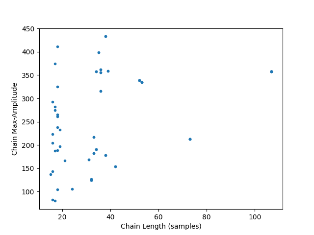
Text(38.347222222222214, 0.5, 'Chain Max-Amplitude')
We can then select the cycle metrics from the cycles in a single chain by specifying the chain index as a condition.
df = C.get_metric_dataframe(conditions='chain_ind==42')
print(df)
Empty DataFrame
Columns: [index, is_good, max_amp, duration, ampSD, DoN, raw_corr, peak_time_ms, trough_time_ms, chain_ind, chain_start, chain_end, chain_len_samples, chain_len_cycles, chain_position, chain_max_amp]
Index: []
Total running time of the script: (0 minutes 0.742 seconds)