Configuring the SIFT

Here we look at how to customise the different parts of the sift algorithm. There are many options which can be customised from top level sift parameters all the way down to extrema detection.

Lets make a simulated signal to get started.

import emd
import numpy as np
import matplotlib.pyplot as plt

sample_rate = 1000
seconds = 10
num_samples = sample_rate*seconds
time_vect = np.linspace(0, seconds, num_samples)
freq = 5

# Change extent of deformation from sinusoidal shape [-1 to 1]
nonlinearity_deg = .25

# Change left-right skew of deformation [-pi to pi]
nonlinearity_phi = -np.pi/4

# Compute the signal
x = emd.utils.abreu2010(freq, nonlinearity_deg, nonlinearity_phi, sample_rate, seconds)
x += np.cos(2*np.pi*1*time_vect)

The SiftConfig object

EMD can create a config dictionary which contains all the options that can be customised for a given sift function. This can be created using the get_config function in the sift submodule. Lets import emd and create the config for a standard sift - we can view the options by calling print on the config.

The SiftConfig dictionary contains all the arguments for functions that are used in the sift algorithm.

• “sift” contains arguments for the high level sift functions such as emd.sift.sift or emd.sift.ensemble_sift
• “imf” contains arguments for emd.sift.get_next_imf
• “envelope” contains arguments for emd.sift.interpolate_envelope
• “extrema”, “mag_pad” and “loc_pad” have arguments for extrema detection and padding

config = emd.sift.get_config('sift')
print(config)

Out:

{'sift_thresh': 1e-08, 'max_imfs': None, 'imf_opts': {}, 'envelope_opts': {}}
sift <class 'emd.sift.SiftConfig'>
sift_thresh : 1e-08
max_imfs : None
imf_opts:
    sd_thresh : 0.1
    env_step_size : 1
envelope_opts:
    interp_method : splrep
extrema_opts:
    pad_width : 2
    parabolic_extrema : False
    mag_pad_opts : {'mode': 'median', 'stat_length': 1}
    loc_pad_opts : {'mode': 'reflect', 'reflect_type': 'odd'}

These arguments are specific for the each type of sift (particularly at the top “sift” level).

config = emd.sift.get_config('ensemble_sift')
print(config)

Out:

{'nensembles': 4, 'ensemble_noise': 0.2, 'noise_mode': 'single', 'nprocesses': 1, 'sift_thresh': 1e-08, 'max_imfs': None, 'imf_opts': {}, 'envelope_opts': {}}
ensemble_sift <class 'emd.sift.SiftConfig'>
nensembles : 4
ensemble_noise : 0.2
noise_mode : single
nprocesses : 1
sift_thresh : 1e-08
max_imfs : None
imf_opts:
    sd_thresh : 0.1
    env_step_size : 1
envelope_opts:
    interp_method : splrep
extrema_opts:
    pad_width : 2
    parabolic_extrema : False
    mag_pad_opts : {'mode': 'median', 'stat_length': 1}
    loc_pad_opts : {'mode': 'reflect', 'reflect_type': 'odd'}

The SiftConfig dictionary contains arguments and default values for functions which are called internally within the different sift implementations. The dictionary can be used to viewing and editing the options before they are passed into the sift function.

The SiftConfig dictionary is nested, in that some items in the dictionary store further dictionaries of options. This hierarchy of options reflects where the options are used in the sift process. The top-level of the dictionary contains arguments which may be passed directly to the sift functions, whilst options needed for internal function calls are stored in nested subdictionaries.

The parameters in the config can be changed in the same way we would change the key-value pairs in a nested dictionary or using a h5py inspiried shorthand.

# This is a top-level argument used directly by ensemble_sift
config['nensembles'] = 24

# This is a sub-arguemnt used by interp_envelope, which is called within
# ensemble_sift.

# Standard
config['envelope_opts']['interp_type'] = 'mono_pchip'
# Shorthard
config['envelope_opts/interp_type'] = 'mono_pchip'

print(config)

Out:

ensemble_sift <class 'emd.sift.SiftConfig'>
nensembles : 24
ensemble_noise : 0.2
noise_mode : single
nprocesses : 1
sift_thresh : 1e-08
max_imfs : None
imf_opts:
    sd_thresh : 0.1
    env_step_size : 1
envelope_opts:
    interp_method : splrep
    interp_type : mono_pchip
extrema_opts:
    pad_width : 2
    parabolic_extrema : False
    mag_pad_opts : {'mode': 'median', 'stat_length': 1}
    loc_pad_opts : {'mode': 'reflect', 'reflect_type': 'odd'}

This nested structure is passed as an unpacked dictionary to our sift function.

config = emd.sift.get_config('sift')
imf = emd.sift.sift(x, **config)

Out:

{'sift_thresh': 1e-08, 'max_imfs': None, 'imf_opts': {}, 'envelope_opts': {}}

Extrema detection and padding

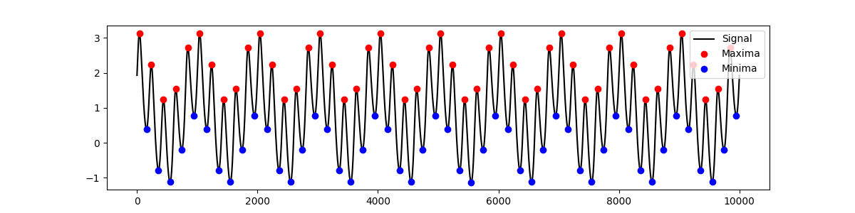
The options are split into six types. Starting from the lowest level, extrema detection and padding in emd is implemented in the emd.sift.find_extrema function. This is a simple function which identifies extrema using the scipy.signal argrelmin and argrelmax functions.

max_locs, max_mag = emd.sift.find_extrema(x)
min_locs, min_mag = emd.sift.find_extrema(x, ret_min=True)

plt.figure(figsize=(12, 3))
plt.plot(x, 'k')
plt.plot(max_locs, max_mag, 'or')
plt.plot(min_locs, min_mag, 'ob')
plt.legend(['Signal', 'Maxima', 'Minima'])

Out:

<matplotlib.legend.Legend object at 0x7f98b3d446d0>

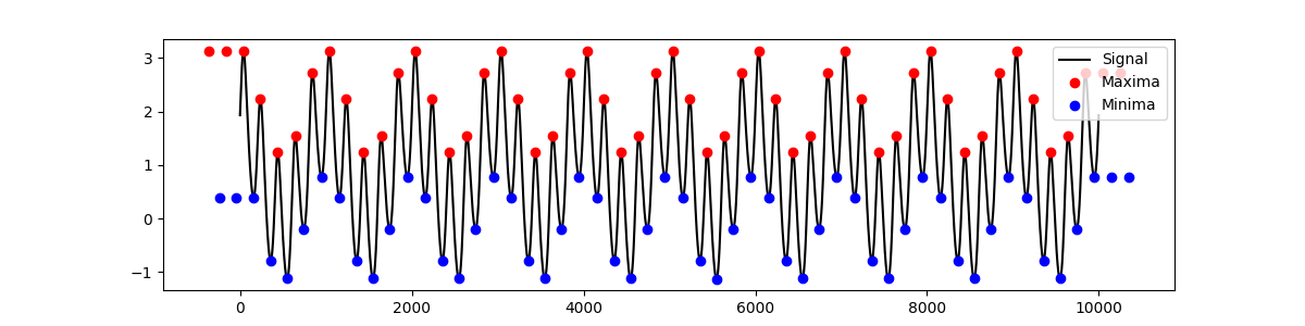
Extrema padding is used to stablise the envelope at the edges of the time-series. The emd.sift.get_padded_extrema function identifies and pads extrema in a time-series. This calls the emd.sift.find_extrema internally.

max_locs, max_mag = emd.sift.get_padded_extrema(x)
min_locs, min_mag = emd.sift.get_padded_extrema(-x)
min_mag = -min_mag

plt.figure(figsize=(12, 3))
plt.plot(x, 'k')
plt.plot(max_locs, max_mag, 'or')
plt.plot(min_locs, min_mag, 'ob')
plt.legend(['Signal', 'Maxima', 'Minima'])

Out:

<matplotlib.legend.Legend object at 0x7f98b3c0fed0>

The extrema detection and padding arguments are specified in the config dict under the extrema, mag_pad and loc_pad keywords. These are passed directly into emd.sift.get_padded_extrema when running the sift.

The padding is controlled by a build in numpy function np.pad. The mag_pad and loc_pad dictionaries are passed into np.pad to define the padding in the y-axis (extrema magnitude) and x-axis (extrema time-point) respectively. Note that np.pad takes a mode as a positional orgument - this must be included as a keyword argument here.

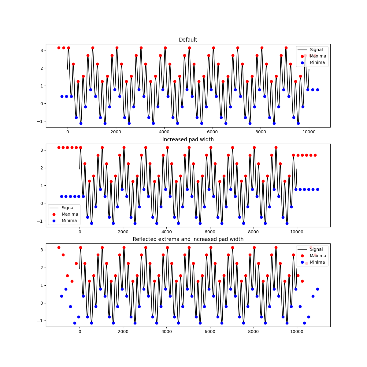
Lets try customising the extrema padding. First we get the ‘extrema’ options from a nested config then try changing a couple of options

ext_opts = config['extrema_opts']

# The default options
max_locs, max_mag = emd.sift.get_padded_extrema(x, **ext_opts)
min_locs, min_mag = emd.sift.get_padded_extrema(-x, **ext_opts)
min_mag = -min_mag

plt.figure(figsize=(12, 12))

plt.subplot(311)
plt.plot(x, 'k')
plt.plot(max_locs, max_mag, 'or')
plt.plot(min_locs, min_mag, 'ob')
plt.legend(['Signal', 'Maxima', 'Minima'])
plt.title('Default')

# Increase the pad width to 5 extrema
ext_opts['pad_width'] = 5
max_locs, max_mag = emd.sift.get_padded_extrema(x, **ext_opts)
min_locs, min_mag = emd.sift.get_padded_extrema(-x, **ext_opts)
min_mag = -min_mag

plt.subplot(312)
plt.plot(x, 'k')
plt.plot(max_locs, max_mag, 'or')
plt.plot(min_locs, min_mag, 'ob')
plt.legend(['Signal', 'Maxima', 'Minima'])
plt.title('Increased pad width')

# Change the y-axis padding to 'reflect' rather than 'median'
ext_opts['mag_pad_opts']['mode'] = 'reflect'
del ext_opts['mag_pad_opts']['stat_length']
max_locs, max_mag = emd.sift.get_padded_extrema(x, **ext_opts)
min_locs, min_mag = emd.sift.get_padded_extrema(-x, **ext_opts)
min_mag = -min_mag

plt.subplot(313)
plt.plot(x, 'k')
plt.plot(max_locs, max_mag, 'or')
plt.plot(min_locs, min_mag, 'ob')
plt.legend(['Signal', 'Maxima', 'Minima'])
plt.title('Reflected extrema and increased pad width')

Out:

Text(0.5, 1.0, 'Reflected extrema and increased pad width')

Envelope interpolation

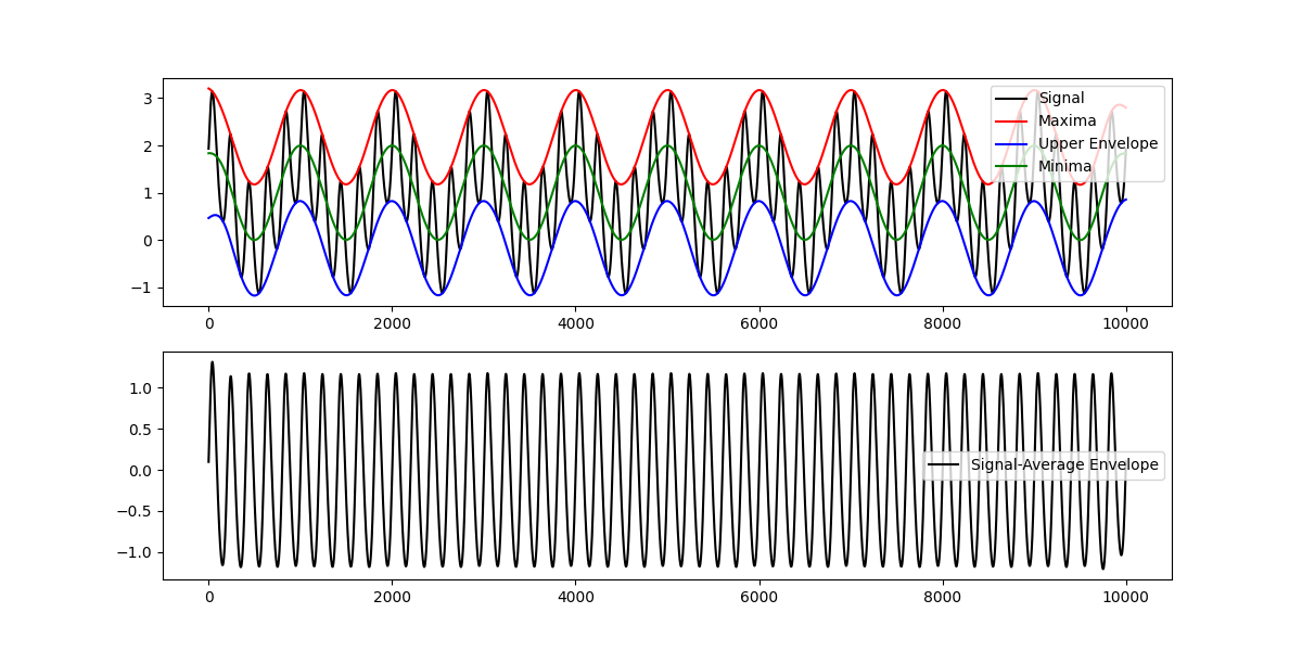
Once extrema have been detected the maxima and minima are interpolated to create an upper and lower envelope. This interpolation is performed with emd.sift.interp_envlope and the options in the envelope section of the config.

This interpolation starts with the padded extrema from the previous section so we will take the envelope and extrema options from the config object

env_opts = config['envelope_opts']

upper_env = emd.utils.interp_envelope(x, mode='upper', **env_opts)
lower_env = emd.utils.interp_envelope(x, mode='lower', **env_opts)
avg_env = (upper_env+lower_env) / 2

plt.figure(figsize=(12, 6))
plt.subplot(211)
plt.plot(x, 'k')
plt.plot(upper_env, 'r')
plt.plot(lower_env, 'b')
plt.plot(avg_env, 'g')
plt.legend(['Signal', 'Maxima', 'Upper Envelope', 'Minima', 'Lower Envelope'])

# Plot the signal with the average of the upper and lower envelopes subtracted.
plt.subplot(212)
plt.plot(x-avg_env, 'k')
plt.legend(['Signal-Average Envelope'])

Out:

<matplotlib.legend.Legend object at 0x7f98b39444d0>

IMF Extraction

The next layer is IMF extraction as implemented in emd.sift.get_next_imf. This uses the envelope interpolation and extrema detection to carry out the sifting iterations on a time-series to return a single intrinsic mode function.

This is the main function used when implementing novel types of sift. For instance, the ensemble sift uses this emd.sift.get_next_imf to extract IMFs from many repetitions of the signal with small amounts of noise added. Similarly the mask sift calls emd.sift.get_next_imf after adding a mask signal to the data.

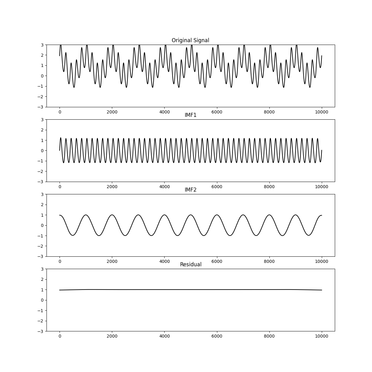
Here we use get_next_imf to implement a very simple sift. We extract the first IMF, subtract it from the data and then extract the second IMF. We then plot the original signal, the two IMFs and the residual.

# Adjust the threshold for accepting an IMF
config['imf_opts/sd_thresh'] = 0.05
# Extract the options for get_next_imf
imf_opts = config['imf_opts']

imf1, continue_sift = emd.sift.get_next_imf(x[:, None], **imf_opts)
print(imf1.shape)
imf2, continue_sift = emd.sift.get_next_imf(x[:, None]-imf1, **imf_opts)

plt.figure(figsize=(12, 12))
plt.subplot(411)
plt.plot(x, 'k')
plt.ylim(-3, 3)
plt.title('Original Signal')

plt.subplot(412)
plt.plot(imf1, 'k')
plt.ylim(-3, 3)
plt.title('IMF1')

plt.subplot(413)
plt.plot(imf2, 'k')
plt.ylim(-3, 3)
plt.title('IMF2')

plt.subplot(414)
plt.plot(x[:, None]-imf1-imf2, 'k')
plt.ylim(-3, 3)
plt.title('Residual')

Out:

(10000, 1)

Text(0.5, 1.0, 'Residual')

Sifting

Finally, the top-level of options configure the sift itself. These options vary between the type of sift that is being performed and many options don’t generalise between different variants of the sift.

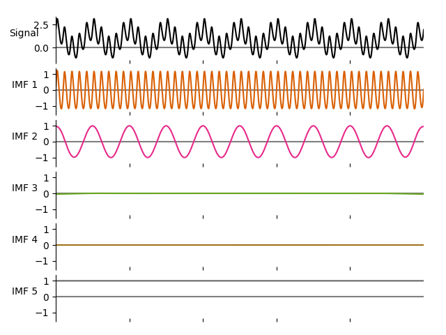
Here we use the config object to perform a simple sift very similar to the one we implemented in the previous section.

config = emd.sift.get_config('sift')

imf = emd.sift.sift(x, **config)

emd.plotting.plot_imfs(imf, cmap=True, scale_y=True)

Out:

{'sift_thresh': 1e-08, 'max_imfs': None, 'imf_opts': {}, 'envelope_opts': {}}