Quick-Start: Running a simple EMD

This getting started tutorial shows how to use EMD to analyse a synthetic signal.

Running an EMD and frequency transform

First of all, we import both the numpy and EMD modules:

# sphinx_gallery_thumbnail_number = 2

import matplotlib.pyplot as plt
import numpy as np
import emd

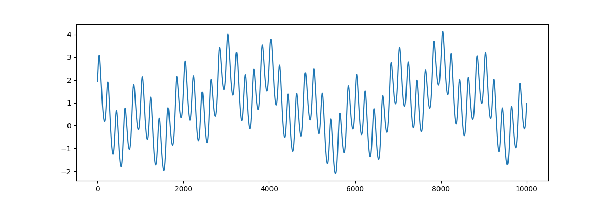
We then define a simulated waveform containing a non-linear wave at 5Hz and a sinusoid at 1Hz:

sample_rate = 1000
seconds = 10
num_samples = sample_rate*seconds

time_vect = np.linspace(0, seconds, num_samples)

freq = 5

# Change extent of deformation from sinusoidal shape [-1 to 1]
nonlinearity_deg = .25

# Change left-right skew of deformation [-pi to pi]
nonlinearity_phi = -np.pi/4

# Compute the signal

# Create a non-linear oscillation
x = emd.utils.abreu2010(freq, nonlinearity_deg, nonlinearity_phi, sample_rate, seconds)

x += np.cos(2 * np.pi * 1 * time_vect)        # Add a simple 1Hz sinusoid
x -= np.sin(2 * np.pi * 2.2e-1 * time_vect)   # Add part of a very slow cycle as a trend

# Visualise the time-series for analysis
plt.figure(figsize=(12, 4))
plt.plot(x)

Out:

[<matplotlib.lines.Line2D object at 0x7fb5f98f8210>]

Try changing the values of nonlinearity_deg and nonlinearity_phi to create different non-sinusoidal waveform shapes.

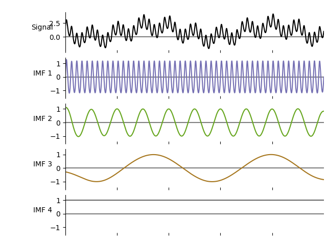
Next, we can then estimate the IMFs for the signal:

imf = emd.sift.sift(x)
print(imf.shape)

Out:

(10000, 4)

and, from the IMFs, compute the instantaneous frequency, phase and amplitude using the Normalised Hilbert Transform Method:

IP, IF, IA = emd.spectra.frequency_transform(imf, sample_rate, 'nht')

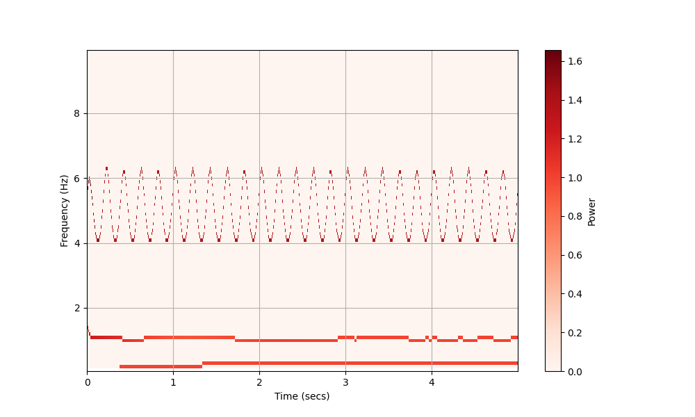
From the instantaneous frequency and amplitude, we can compute the Hilbert-Huang spectrum:

freq_edges, freq_bins = emd.spectra.define_hist_bins(0, 10, 100)
hht = emd.spectra.hilberthuang(IF, IA, freq_edges)

Visualising the results

we can now plot some summary information, first the IMFs:

emd.plotting.plot_imfs(imf, scale_y=True, cmap=True)

and now the Hilbert-Huang transform of this decomposition

plt.figure(figsize=(10, 6))

plt.subplot(1, 1, 1)
plt.pcolormesh(time_vect[:5000], freq_bins, hht[:, :5000], cmap='Reds')
cb = plt.colorbar()
cb.set_label('Power')
plt.ylabel('Frequency (Hz)')
plt.xlabel('Time (secs)')

plt.grid(True)

Out:

/home/docs/checkouts/readthedocs.org/user_builds/emd/checkouts/v0.3.2/doc/source/tutorials/00_quick_start/emd_tutorial_00_start_01_quicksift.py:84: MatplotlibDeprecationWarning: shading='flat' when X and Y have the same dimensions as C is deprecated since 3.3.  Either specify the corners of the quadrilaterals with X and Y, or pass shading='auto', 'nearest' or 'gouraud', or set rcParams['pcolor.shading'].  This will become an error two minor releases later.
  plt.pcolormesh(time_vect[:5000], freq_bins, hht[:, :5000], cmap='Reds')