Masked sifting

This tutorial introduces some of the issues that standard EMD algorithms can have with intermitent signals and shows how the Masked sift can resolve them.

Lets make a simulated signal to get started.

import emd
import numpy as np
import matplotlib.pyplot as plt

seconds = 5
sample_rate = 1024
time_vect = np.linspace(0, seconds, seconds*sample_rate)

# Create an amplitude modulation
am = np.sin(2*np.pi*time_vect)
am[am < 0] = 0

# Create a 25Hz signal and introduce the amplitude modulation
xx = am*np.sin(2*np.pi*25*time_vect)

# Create a non-modulated 6Hz signal
yy = .5*np.sin(2*np.pi*6*time_vect)

# Sum the 25Hz and 6Hz components together
xy = xx+yy

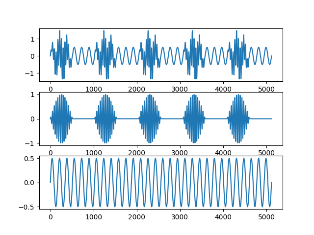
# Make a quick summary plot
plt.figure()
plt.subplot(311)
plt.plot(xy)
plt.subplot(312)
plt.plot(xx)
plt.subplot(313)
plt.plot(yy)

# sphinx_gallery_thumbnail_number = 2

Out:

[<matplotlib.lines.Line2D object at 0x7f88f24bd890>]

This signal doesn’t contain any noise and only has two frequency components so should be straightforward to sift. Unfortunately, as the 25Hz signal component disappears completely for parts of the signal the EMD doesn’t quite do what we’d want it to.

Here we run a default sift and plot the IMFs.

imf = emd.sift.sift(xy, max_imfs=3)
emd.plotting.plot_imfs(imf, cmap=True, scale_y=True)

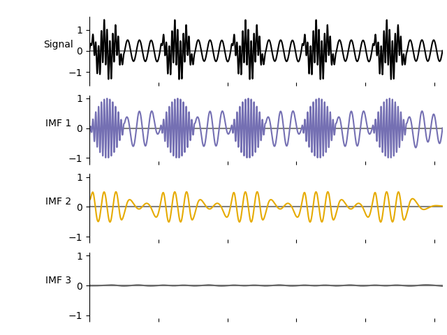
The signals are well separated when both oscillations are present. However in

time periods where the fast 25Hz signal disappears the slower signal jumps up to become part of the fast component. We’d prefer the separation into narrow band components as seen in the simulations above…

This happens as EMD is a locally adaptive algorithm - the peaks and troughs in the signal define the time-scales that are analysed for a given part of the signal. So, the first IMF will always find the fastest peaks for every part of the signal even if the definition of ‘fast’ might be different in different segments.

The Masked sift is a potential solution to this problem. This is a simple trick which effectively puts a lower bound on the frequency content that can enter a particular IMF. We will add a known masking signal to our time-series before running emd.sift.get_next_imf. Any signals which are lower in frequency than this mask should then be ignored by the sift in favour of this known signal. Finally, we can remove the known mask to recover our IMF.

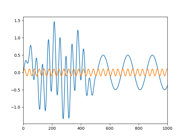
 Here we make a 30Hz mask and plot it next to a segment of our time-series.

mask = 0.1*np.sin(2*np.pi*30*time_vect)

plt.figure()
plt.plot(xy)
plt.plot(mask)
plt.xlim(0, 1000)

Out:

(0.0, 1000.0)

We see that the masking signal is close in frequency to the fast burst but much faster than the 6Hz signal.

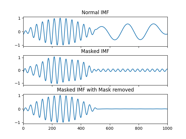
Next we identify our next IMF on the raw signal with and without the mask

imf_raw, _ = emd.sift.get_next_imf(xy)
imf_mask, _ = emd.sift.get_next_imf(xy+mask)

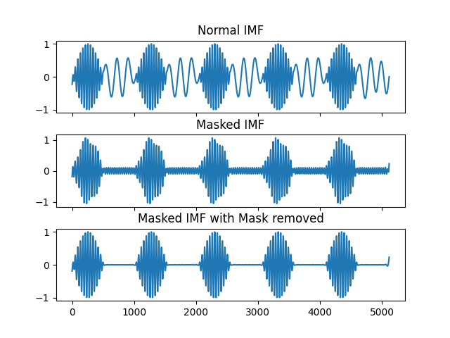
The normal IMF in the top panel has the problem we saw earlier, the slow signal is leaking into the fast IMF. The masked IMF successfully suppresses this slow signal, replacing it with the mask frequency. Finally, subtracting the mask removes everything but the 25Hz oscillation which now correctly disappears between bursts.

plt.figure()
plt.subplots_adjust(hspace=0.3)
plt.subplot(311)
plt.plot(imf_raw)
plt.xlim(0, 1000)
plt.title('Normal IMF')
plt.gca().set_xticklabels([])
plt.subplot(312)
plt.plot(imf_mask)
plt.xlim(0, 1000)
plt.title('Masked IMF')
plt.gca().set_xticklabels([])
plt.subplot(313)
plt.plot(imf_mask - mask[:, np.newaxis])
plt.xlim(0, 1000)
plt.title('Masked IMF with Mask removed')

Out:

Text(0.5, 1.0, 'Masked IMF with Mask removed')

This effect is more obvious if we look at the whole time-courses without zooming in

plt.figure()
plt.subplots_adjust(hspace=0.3)
plt.subplot(311)
plt.plot(imf_raw)
plt.title('Normal IMF')
plt.gca().set_xticklabels([])
plt.subplot(312)
plt.plot(imf_mask)
plt.title('Masked IMF')
plt.gca().set_xticklabels([])
plt.subplot(313)
plt.plot(imf_mask - mask[:, np.newaxis])
plt.title('Masked IMF with Mask removed')

Out:

Text(0.5, 1.0, 'Masked IMF with Mask removed')

This masking process is implemented in emd.sift.get_next_imf_mask which works much like emd.sift.get_next_imf with a couple of extra options for adding masks. We can specify the frequency and amplitude of the mask to be applied whilst isolating our IMF.

It is important that the mask frequency is approximately equal to the signal component we want to isolate. If we use a mask of too high or too low frequency then the procedure will not work.

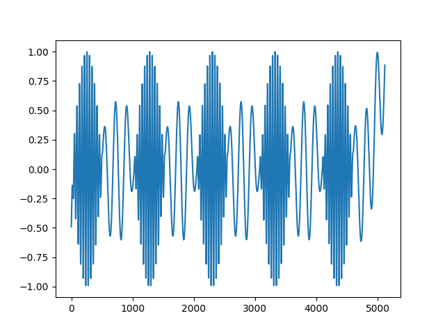
Next we use a mask with an very high frequency which suppresses both signal components.

# Masks should be specified in normalised frequencies between 0 and .5 where 0.5 is half the sampling rate
high_mask_freq = 150/sample_rate
imf_high_mask, _ = emd.sift.get_next_imf_mask(xy, high_mask_freq, 2)

plt.figure()
plt.plot(imf_high_mask)

Out:

[<matplotlib.lines.Line2D object at 0x7f88f2605c90>]

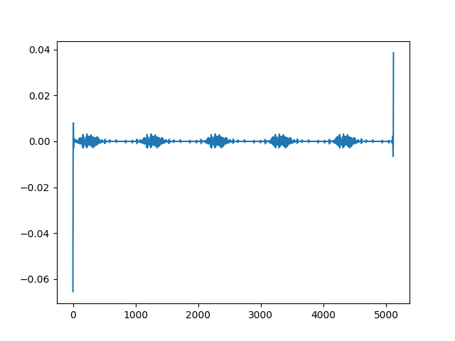
Finally a very low frequency mask which allows both components back through…

low_mask_freq = 2/sample_rate
imf_low_mask, _ = emd.sift.get_next_imf_mask(xy, low_mask_freq, 2)


plt.figure()
plt.plot(imf_low_mask)

Out:

[<matplotlib.lines.Line2D object at 0x7f88f23a5110>]

emd.sift.mask_sift uses emd.sift.get_next_imf_mask internally to run a whole set of sifts using the masking method. Each IMF is isolated with a separate mask which decreases in frequency for each successive IMF.

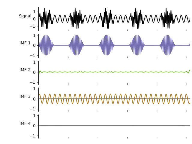
Here we run a mask_sift using mask frequencies starting at 30Hz. This will reduce by one half for each successive IMF - the second mask will be 15Hz, the third is 7.5Hz and so on.

imf, mask_freqs = emd.sift.mask_sift(xy, mask_freqs=30/sample_rate, ret_mask_freq=True, max_imfs=4)

print(mask_freqs * sample_rate)

Out:

[30.   15.    7.5   3.75]

We can see that this sift nicely separates the two components. The first IMF contains the 25Hz bursting signal which returns to a flat line between events. The second IMF contains very low amplitude noise. This is as the mask frequency of 15Hz for the second mask is still too high to isolate the oscillation of 6Hz - so IMF 2 is essentially flat. The third IMF with a mask frequency of 7.5Hz is about right to isolate the 6Hz signal.

emd.plotting.plot_imfs(imf, cmap=True, scale_y=True)