The sift in detail

Here, we will run through the different steps of the sift and get to know some of the lower-level functions which are used by the core sift functions. There are four levels of functions which are used in the sift.

We will take a look at each of these steps in turn using a simulated time-series.

Lets make a simulated signal to get started.

import emd
import numpy as np
import matplotlib.pyplot as plt

sample_rate = 1000
seconds = 10
num_samples = sample_rate*seconds
time_vect = np.linspace(0, seconds, num_samples)
freq = 5

# Change extent of deformation from sinusoidal shape [-1 to 1]
nonlinearity_deg = .25

# Change left-right skew of deformation [-pi to pi]
nonlinearity_phi = -np.pi/4

# Create a non-linear oscillation
x = emd.utils.abreu2010(freq, nonlinearity_deg, nonlinearity_phi, sample_rate, seconds)

x += np.cos(2 * np.pi * 1 * time_vect)        # Add a simple 1Hz sinusoid
x -= np.sin(2 * np.pi * 2.2e-1 * time_vect)   # Add part of a very slow cycle as a trend

# sphinx_gallery_thumbnail_number = 4

Sifting

The top-level of options configure the sift itself. These options vary between the type of sift that is being performed and options don’t generalise between different variants of the sift.

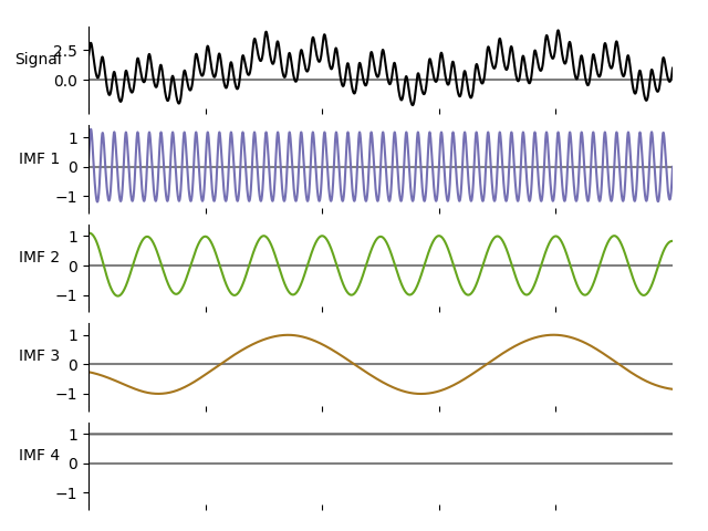
Here we will run a standard sift on our simulation.

# Get the default configuration for a sift
config = emd.sift.get_config('sift')
# Adjust the threshold for accepting an IMF
config['imf_opts/sd_thresh'] = 0.05

imf = emd.sift.sift(x)

emd.plotting.plot_imfs(imf, cmap=True, scale_y=True)

Internally the sift function

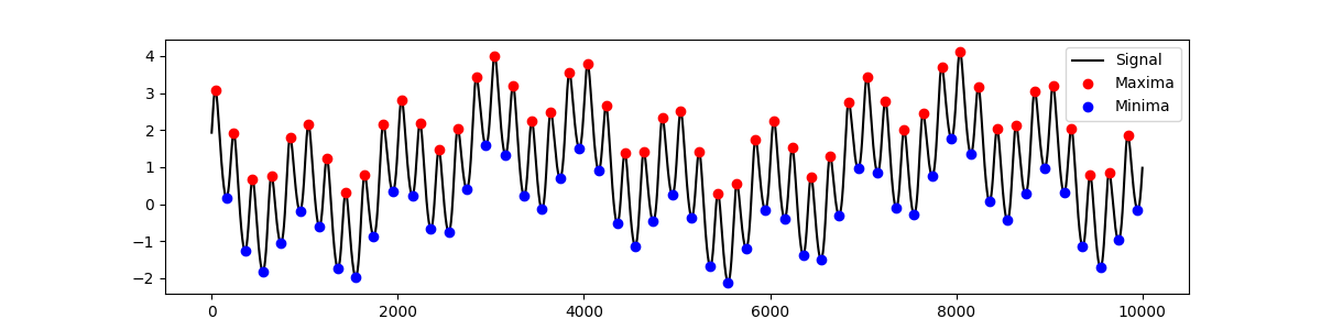
Extrema detection and padding

The options are split into six types. Starting from the lowest level, extrema detection and padding in emd is implemented in the emd.sift.find_extrema function. This is a simple function which identifies extrema using the scipy.signal argrelmin and argrelmax functions.

max_locs, max_mag = emd.sift.find_extrema(x)
min_locs, min_mag = emd.sift.find_extrema(x, ret_min=True)

plt.figure(figsize=(12, 3))
plt.plot(x, 'k')
plt.plot(max_locs, max_mag, 'or')
plt.plot(min_locs, min_mag, 'ob')
plt.legend(['Signal', 'Maxima', 'Minima'])

Out:

<matplotlib.legend.Legend object at 0x7f9f50e3cfd0>

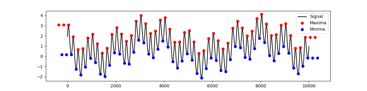
Extrema padding is used to stablise the envelope at the edges of the time-series. The emd.sift.get_padded_extrema function identifies and pads extrema in a time-series. This calls the emd.sift.find_extrema internally.

max_locs, max_mag = emd.sift.get_padded_extrema(x)
min_locs, min_mag = emd.sift.get_padded_extrema(-x)
min_mag = -min_mag

plt.figure(figsize=(12, 3))
plt.plot(x, 'k')
plt.plot(max_locs, max_mag, 'or')
plt.plot(min_locs, min_mag, 'ob')
plt.legend(['Signal', 'Maxima', 'Minima'])

Out:

<matplotlib.legend.Legend object at 0x7f9f50bc6950>

The extrema detection and padding arguments are specified in the config dict under the extrema, mag_pad and loc_pad keywords. These are passed directly into emd.sift.get_padded_extrema when running the sift.

The padding is controlled by a build in numpy function np.pad. The mag_pad and loc_pad dictionaries are passed into np.pad to define the padding in the y-axis (extrema magnitude) and x-axis (extrema time-point) respectively. Note that np.pad takes a mode as a positional orgument - this must be included as a keyword argument here.

Lets try customising the extrema padding. First we get the ‘extrema’ options from a nested config then try changing a couple of options

ext_opts = config['extrema_opts']

# The default options
max_locs, max_mag = emd.sift.get_padded_extrema(x, **ext_opts)
min_locs, min_mag = emd.sift.get_padded_extrema(-x, **ext_opts)
min_mag = -min_mag

plt.figure(figsize=(12, 12))

plt.subplot(311)
plt.plot(x, 'k')
plt.plot(max_locs, max_mag, 'or')
plt.plot(min_locs, min_mag, 'ob')
plt.legend(['Signal', 'Maxima', 'Minima'])
plt.title('Default')

# Increase the pad width to 5 extrema
ext_opts['pad_width'] = 5
max_locs, max_mag = emd.sift.get_padded_extrema(x, **ext_opts)
min_locs, min_mag = emd.sift.get_padded_extrema(-x, **ext_opts)
min_mag = -min_mag

plt.subplot(312)
plt.plot(x, 'k')
plt.plot(max_locs, max_mag, 'or')
plt.plot(min_locs, min_mag, 'ob')
plt.legend(['Signal', 'Maxima', 'Minima'])
plt.title('Increased pad width')

# Change the y-axis padding to 'reflect' rather than 'median'
ext_opts['mag_pad_opts']['mode'] = 'reflect'
del ext_opts['mag_pad_opts']['stat_length']
max_locs, max_mag = emd.sift.get_padded_extrema(x, **ext_opts)
min_locs, min_mag = emd.sift.get_padded_extrema(-x, **ext_opts)
min_mag = -min_mag

plt.subplot(313)
plt.plot(x, 'k')
plt.plot(max_locs, max_mag, 'or')
plt.plot(min_locs, min_mag, 'ob')
plt.legend(['Signal', 'Maxima', 'Minima'])
plt.title('Reflected extrema and increased pad width')

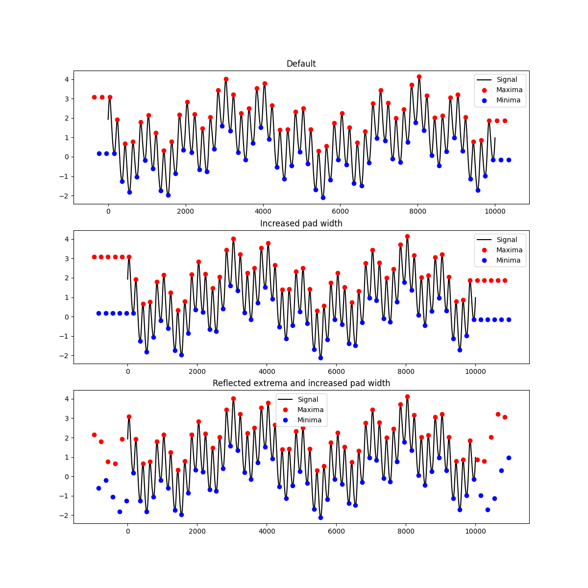
Out:

Text(0.5, 1.0, 'Reflected extrema and increased pad width')

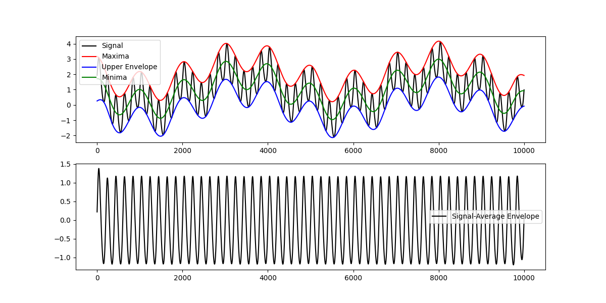
Envelope interpolation

Once extrema have been detected the maxima and minima are interpolated to create an upper and lower envelope. This interpolation is performed with emd.sift.interp_envlope and the options in the envelope section of the config.

This interpolation starts with the padded extrema from the previous section so we will take the envelope and extrema options from the config object

env_opts = config['envelope_opts']

upper_env = emd.utils.interp_envelope(x, mode='upper', **env_opts)
lower_env = emd.utils.interp_envelope(x, mode='lower', **env_opts)
avg_env = (upper_env+lower_env) / 2

plt.figure(figsize=(12, 6))
plt.subplot(211)
plt.plot(x, 'k')
plt.plot(upper_env, 'r')
plt.plot(lower_env, 'b')
plt.plot(avg_env, 'g')
plt.legend(['Signal', 'Maxima', 'Upper Envelope', 'Minima', 'Lower Envelope'])

# Plot the signal with the average of the upper and lower envelopes subtracted.
plt.subplot(212)
plt.plot(x-avg_env, 'k')
plt.legend(['Signal-Average Envelope'])

Out:

<matplotlib.legend.Legend object at 0x7f9f508d3c50>

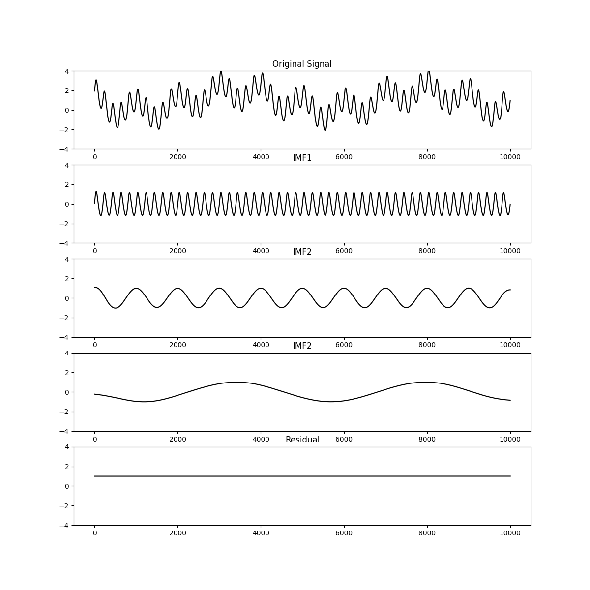
IMF Extraction

The next layer is IMF extraction as implemented in emd.sift.get_next_imf. This uses the envelope interpolation and extrema detection to carry out the sifting iterations on a time-series to return a single intrinsic mode function.

This is the main function used when implementing novel types of sift. For instance, the ensemble sift uses this emd.sift.get_next_imf to extract IMFs from many repetitions of the signal with small amounts of noise added. Similarly the mask sift calls emd.sift.get_next_imf after adding a mask signal to the data.

Here we use get_next_imf to implement a very simple sift. We extract the first IMF, subtract it from the data and then extract the second and third IMFs. We then plot the original signal, the IMFs and the residual.

# Extract the options for get_next_imf
imf_opts = config['imf_opts']

imf1, continue_sift = emd.sift.get_next_imf(x[:, None],           **imf_opts)
imf2, continue_sift = emd.sift.get_next_imf(x[:, None]-imf1,      **imf_opts)
imf3, continue_sift = emd.sift.get_next_imf(x[:, None]-imf1-imf2, **imf_opts)

plt.figure(figsize=(12, 12))
plt.subplot(511)
plt.plot(x, 'k')
plt.ylim(-4, 4)
plt.title('Original Signal')

plt.subplot(512)
plt.plot(imf1, 'k')
plt.ylim(-4, 4)
plt.title('IMF1')

plt.subplot(513)
plt.plot(imf2, 'k')
plt.ylim(-4, 4)
plt.title('IMF2')

plt.subplot(514)
plt.plot(imf3, 'k')
plt.ylim(-4, 4)
plt.title('IMF2')

plt.subplot(515)
plt.plot(x[:, None]-imf1-imf2-imf3, 'k')
plt.ylim(-4, 4)
plt.title('Residual')

Out:

Text(0.5, 1.0, 'Residual')