The Holospectrum

This tutorial shows how we can compute a holospectrum to characterise the distribution of power in a signal as a function of both frequency of the carrier wave and the frequency of any amplitude modulations

Simulating and exploring amplitude modulations

First of all, we import EMD alongside numpy and matplotlib. We will also use scipy’s ndimage module to smooth our results for visualisation later.

# sphinx_gallery_thumbnail_number = 5

import matplotlib.pyplot as plt
from scipy import ndimage
import numpy as np
import emd

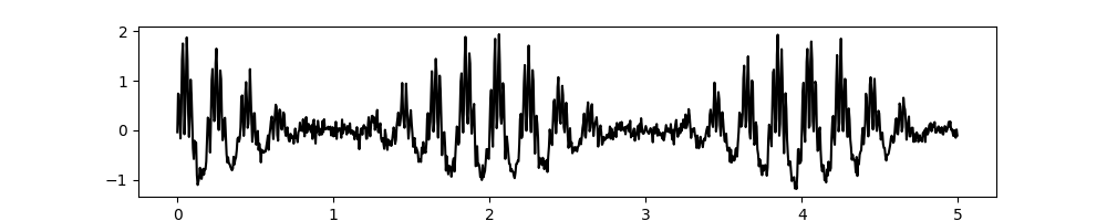
First we create a simulated signal to analyse. This signal will be composed of a linear trend and two oscillations, each with a different amplitude modulation.

seconds = 60
sample_rate = 200
t = np.linspace(0, seconds, seconds*sample_rate)

# First we create a slow 4.25Hz oscillation with a 0.5Hz amplitude modulation
slow = np.sin(2*np.pi*5*t) * (.5+(np.cos(2*np.pi*.5*t)/2))

# Second, we create a faster 37Hz oscillation that is amplitude modulated by the first.
fast = .5*np.sin(2*np.pi*37*t) * (slow+(.5+(np.cos(2*np.pi*.5*t)/2)))

# We create our signal by summing the oscillation and adding some noise
x = slow+fast + np.random.randn(*t.shape)*.1

# Plot the first 5 seconds of data
plt.figure(figsize=(10, 2))
plt.plot(t[:sample_rate*5], x[:sample_rate*5], 'k')

Out:

[<matplotlib.lines.Line2D object at 0x7f9f4f963850>]

Next we run a simple sift with a cubic spline interpolation and estimate the instantaneous frequency statistics from it using the Normalised Hilbert Transform

config = emd.sift.get_config('mask_sift')
config['max_imfs'] = 7
config['mask_freqs'] = 50/sample_rate
config['mask_amp_mode'] = 'ratio_sig'
config['imf_opts/sd_thresh'] = 0.05
imf = emd.sift.mask_sift(x, **config)
IP, IF, IA = emd.spectra.frequency_stats(imf, sample_rate, 'nht')

# Visualise the IMFs
emd.plotting.plot_imfs(imf[:sample_rate*5, :], cmap=True, scale_y=True)

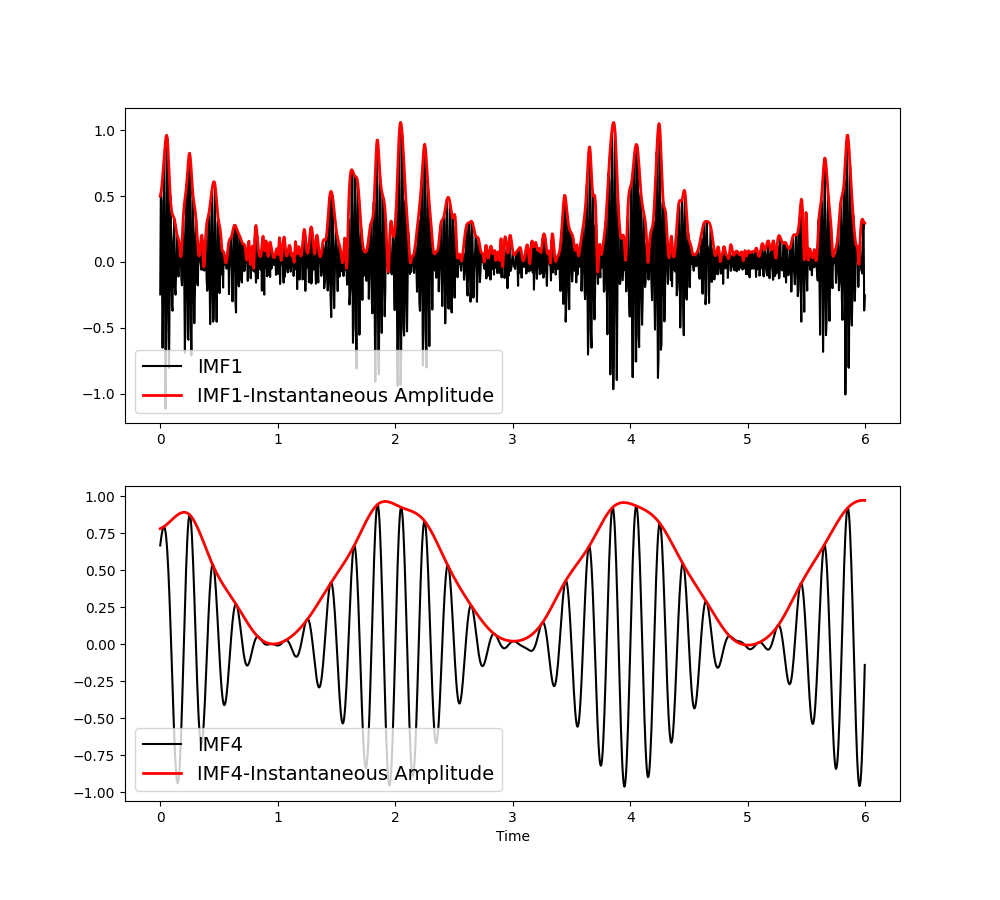
The first IMF contains the 30Hz oscillation and the fourth captures the 8Hz oscillation. Their amplitude modulations are described in the IA (Instantaneous Amplitude) variable. We can visualise these, note that the amplitude modulations (in red) are themselves oscillatory.

plt.figure(figsize=(10, 9))
plt.subplot(211)
plt.plot(t[:sample_rate*6], imf[:sample_rate*6, 0], 'k')
plt.plot(t[:sample_rate*6], IA[:sample_rate*6, 0], 'r', linewidth=2)
plt.legend(['IMF1', 'IMF1-Instantaneous Amplitude'], fontsize=14)
plt.subplot(212)
plt.plot(t[:sample_rate*6], imf[:sample_rate*6, 3], 'k')
plt.plot(t[:sample_rate*6], IA[:sample_rate*6, 3], 'r', linewidth=2)
plt.legend(['IMF4', 'IMF4-Instantaneous Amplitude'], fontsize=14)
plt.xlabel('Time')

Out:

Text(0.5, 69.7222222222222, 'Time')

We can describe the frequency content of these amplitude modulation signal with another EMD. This is called a second level sift which decomposes the instantaneous amplitude of each first level IMF with an additional set of IMFs.

# Helper function for the second level sift
def mask_sift_second_layer(IA, masks, config={}):
    imf2 = np.zeros((IA.shape[0], IA.shape[1], config['max_imfs']))
    for ii in range(IA.shape[1]):
        config['mask_freqs'] = masks[ii:]
        tmp = emd.sift.mask_sift(IA[:, ii], **config)
        imf2[:, ii, :tmp.shape[1]] = tmp
    return imf2


# Define sift parameters for the second level
masks = np.array([25/2**ii for ii in range(12)])/sample_rate
config = emd.sift.get_config('mask_sift')
config['mask_amp_mode'] = 'ratio_sig'
config['mask_amp'] = 2
config['max_imfs'] = 5
config['imf_opts/sd_thresh'] = 0.05
config['envelope_opts/interp_method'] = 'mono_pchip'

# Sift the first 5 first level IMFs
imf2 = mask_sift_second_layer(IA, masks, config=config)

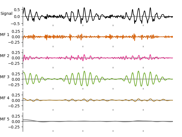
We can see that the oscillatory content in the amplitude modulations has been described with ad additional set of IMFs. Here we plot the IMFs for the amplitude modulations of IMFs 1 (as plotted above).

emd.plotting.plot_imfs(imf2[:sample_rate*5, 0, :], scale_y=True, cmap=True)

We can compute the frequency stats for the second level IMFs using the same options as for the first levels.

IP2, IF2, IA2 = emd.spectra.frequency_stats(imf2, sample_rate, 'nht')

Finally, we want to visualise our results. We first define two sets of histogram bins, one for the main carrier frequency oscillations and one for the amplitude modulations.

# Carrier frequency histogram definition
edges, bins = emd.spectra.define_hist_bins(1, 100, 128, 'log')
# AM frequency histogram definition
edges2, bins2 = emd.spectra.define_hist_bins(1e-2, 32, 64, 'log')

# Compute the 1d Hilbert-Huang transform (power over carrier frequency)
spec = emd.spectra.hilberthuang_1d(IF, IA, edges)

# Compute the 2d Hilbert-Huang transform (power over time x carrier frequency)
hht = emd.spectra.hilberthuang(IF, IA, edges)
shht = ndimage.gaussian_filter(hht, 2)

# Compute the 3d Holospectrum transform (power over time x carrier frequency x AM frequency)
# Here we return the time averaged Holospectrum (power over carrier frequency x AM frequency)
holo = emd.spectra.holospectrum(IF[:, :], IF2[:, :, :], IA2[:, :, :], edges, edges2)
sholo = holo

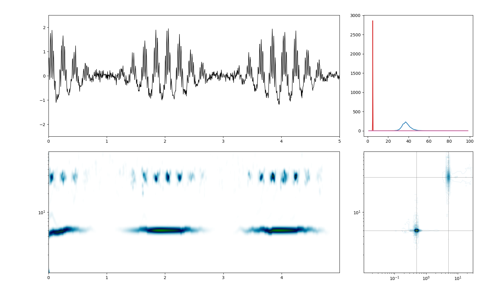
We summarise the results with a four part figure: - top-left shows a segment of our original signal - top-right shows the 1D Hilbert-Huang power spectrum - bottom-left shows a segment of the 2D Hilbert-Huang transform - bottom-right shows the Holospectrum summed over the time dimension

plt.figure(figsize=(16, 10))

# Plot a section of the time-course
plt.axes([.1, .55, .6, .4])
plt.plot(t[:sample_rate*5], x[:sample_rate*5], 'k', linewidth=1)
plt.xlim(0, 5)
plt.ylim(-2.5, 2.5)

# Plot a section of the time-course
plt.axes([.75, .55, .225, .4])
plt.plot(bins, spec)

# Plot a section of the Hilbert-Huang transform
plt.axes([.1, .1, .6, .4])
plt.pcolormesh(t[:sample_rate*5], bins, shht[:, :sample_rate*5], cmap='ocean_r')
plt.yscale('log')

# Plot a the Holospectrum
plt.axes([.75, .1, .225, .4])
#plt.pcolormesh(bins2, bins, sholo.T, cmap='ocean_r')
plt.contour(bins2, bins, np.sqrt(sholo.T), 48, cmap='ocean_r')
plt.yscale('log')
plt.xscale('log')
plt.plot((bins2[0], bins2[-1]), (5, 5), 'grey', linewidth=.5)
plt.plot((bins2[0], bins2[-1]), (37, 37), 'grey', linewidth=.5)
plt.plot((.5, .5), (bins[0], bins[-1]), 'grey', linewidth=.5)
plt.plot((5, 5), (bins[0], bins[-1]), 'grey', linewidth=.5)

Out:

/home/docs/checkouts/readthedocs.org/user_builds/emd/checkouts/v0.3.1/doc/source/tutorials/02_spectrum_analysis/plot_tutorial2.py:164: MatplotlibDeprecationWarning: shading='flat' when X and Y have the same dimensions as C is deprecated since 3.3.  Either specify the corners of the quadrilaterals with X and Y, or pass shading='auto', 'nearest' or 'gouraud', or set rcParams['pcolor.shading'].  This will become an error two minor releases later.
  plt.pcolormesh(t[:sample_rate*5], bins, shht[:, :sample_rate*5], cmap='ocean_r')

[<matplotlib.lines.Line2D object at 0x7f9f508a8e50>]