Note
Go to the end to download the full example code
Cycle detection from IMFs#
Here we will use the ‘cycle’ submodule of EMD to identify and analyse individual cycles of an oscillatory signal
Simulating a noisy signal#
Firstly we will import emd and simulate a signal
import emd
import numpy as np
import matplotlib.pyplot as plt
# Define and simulate a simple signal
peak_freq = 15
sample_rate = 256
seconds = 10
noise_std = .4
x = emd.simulate.ar_oscillator(peak_freq, sample_rate, seconds,
noise_std=noise_std, random_seed=42, r=.96)[:, 0]
t = np.linspace(0, seconds, seconds*sample_rate)
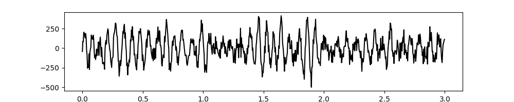
# Plot the first 5 seconds of data
plt.figure(figsize=(10, 2))
plt.plot(t[:sample_rate*3], x[:sample_rate*3], 'k')
# sphinx_gallery_thumbnail_number = 5
[<matplotlib.lines.Line2D object at 0x7f0ebb012650>]
Extract IMFs & find cycles#
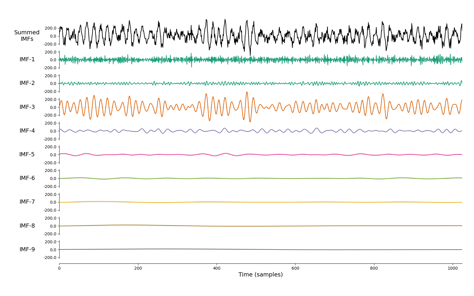
We next run a mask sift with the default parameters to isolate the 15Hz oscillation. There is only one clear oscillatory signal in this simulation. This is extracted in IMF-3 whilst the remaining IMFs contain low-amplitude noise.
# Run a mask sift
imf = emd.sift.mask_sift(x)

# Visualise the IMFs
emd.plotting.plot_imfs(imf[:sample_rate*4, :])
<Axes: xlabel='Time (samples)'>
Next, we want to identify single cycles of any oscillations that are present in our IMFs. There are many ways to do this depending on the signal and signal-features of interest. The EMD package provides a method which extract cycle locations based on the instantaneous phase of an IMF. In its simplest form this will detect successive cycles within the IMF, though we can also run some additional checks to reject ‘bad’ cycles or specify time-periods to exclude from the cycle detection.
Will will run through some examples of these in the next couple of sections.
First, we compute the instantaneous phase of our IMFs using the
frequency_transform function before detecting cycle indices from the IP
using get_cycle_vector.
The detection is based on finding large jumps in the instantaneous phase of
each IMF. By default, we will consider any phase jump greater than 1.5*pi as
a boundary between two cycles. This can be customised using the
phase_step argument in get_cycle_vector.
We can optionally run a set of tests on the detected cycles to remove ‘bad’
cycles from the analysis at an early stage. We will go into more detail into
this later, for now we will run the function to get all_cycles.
# Compute frequency domain features using the normalised-Hilbert transform
IP, IF, IA = emd.spectra.frequency_transform(imf, sample_rate, 'nht')

# Extract cycle locations
all_cycles = emd.cycles.get_cycle_vector(IP, return_good=False)

# ``all_cycles`` is an array of the same size as the input instantaneous phase.
# Each row contains a vector of itegers indexing the location of successive
# cycles for that IMF.

print('Input IMF shape is - {0}'.format(IP.shape))
print('Input all_cycles shape is - {0}'.format(all_cycles.shape))
Input IMF shape is - (2560, 9)
Input all_cycles shape is - (2560, 9)
For each IMF, all_cycles stores either a zero or an integer greater than
zero for each time sample. A value zero indicates that no cycle is occurring
at that time (perhaps as it has been excluded by our cycle quality checks in
the next section) whilst a non-zero value indicates that that time-sample
belongs to a specific cycle.
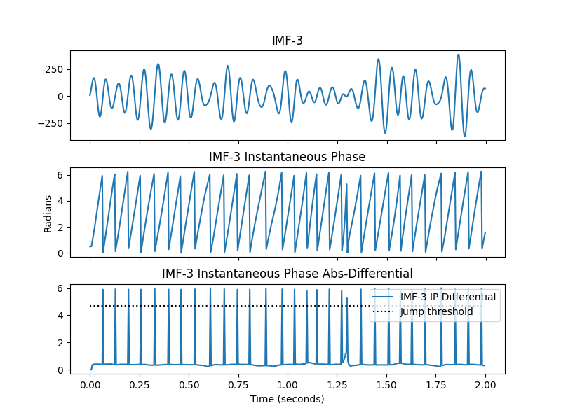
# Firstly, cycles  are detected by looking for phase 'jumps' where the phase
# resets between cycles.  The default threshold for a jump is 1.5*pi. Let's
# take a look at this in IMF-3

plt.figure(figsize=(8, 6))
plt.subplots_adjust(hspace=0.3)
plt.subplot(311)
plt.plot(t[:sample_rate*2], imf[:sample_rate*2, 2])
plt.gca().set_xticklabels([])
plt.title('IMF-3')
plt.subplot(312)
plt.plot(t[:sample_rate*2], IP[:sample_rate*2, 2])
plt.title('IMF-3 Instantaneous Phase')
plt.ylabel('Radians')
plt.gca().set_xticklabels([])
plt.subplot(313)
plt.plot(t[1:sample_rate*2], np.abs(np.diff(IP[:sample_rate*2, 2])))
plt.plot((0, 2), (1.5*np.pi, 1.5*np.pi), 'k:')
plt.xlabel('Time (seconds)')
plt.title('IMF-3 Instantaneous Phase Abs-Differential')
plt.legend(['IMF-3 IP Differential', 'Jump threshold'], loc='upper right')
<matplotlib.legend.Legend object at 0x7f0eb9549310>
We can see that the large phase jumps occur at the ascending zero-crossing of each cycle. In a clear signal, these are very simple to detect using a blunt threshold.
What makes a ‘good’ cycle?#
There are many methods for detecting oscillatory cycles within a signal. Here we provide one approach for identifying whether a signal contains clear and interpretable cycles based on analysis of its instantaneous phase. This process takes the cycles detected by the phase jumps and runs four additional checks.
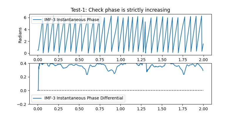
We define a ‘good’ cycle as one with:
A strictly positively increasing phase
A phase starting within phase_step of zero ie the lowest value of IP must be less than phase_step
A phase ending within phase_step of 2pi the highest value of IP must be between 2pi and 2pi-phase_step
A set of 4 unique control points (ascending zero, peak, descending zero & trough)
Lets take a look at these checks in IMF-3. Firstly, we run test 1:
# We use the unwrapped phased so we don't have to worry about jumps between cycles
unwrapped_phase = np.diff(np.unwrap(IP[:sample_rate*2, 2]))

# Plot the differential of the unwrapped phasee
plt.figure(figsize=(8, 4))
plt.subplot(211)
plt.plot(t[:sample_rate*2], IP[:sample_rate*2, 2])
plt.legend(['IMF-3 Instantaneous Phase'])
plt.ylabel('Radians')
plt.title('Test-1: Check phase is strictly increasing')
plt.subplot(212)
plt.plot(t[1:sample_rate*2], unwrapped_phase)
plt.plot((0, 2), (0, 0), 'k:')
plt.ylim(-.2, .4)
plt.legend(['IMF-3 Instantaneous Phase Differential'])
<matplotlib.legend.Legend object at 0x7f0ebb009310>
We can see that the instantaneous phase of most cycles is positive throughout the cycle. Only one cycle (around 1.6 seconds into the simulation) has negative values which correspond to a reversal in the normal wrapped IP.
The second test looks to make sure that each cycles phase covers the whole 2pi range. If the phase doesn’t reach these limits it indicates that a phase jump occurred early or late in the cycle (for instance we might have a peak which is below zero in the raw time-course) leaving an incomplete oscillation.
plt.figure(figsize=(8, 4))
plt.title('Tests 2+3: Check phase covers the full 2pi range')
plt.plot(t[:sample_rate*2], IP[:sample_rate*2, 2], label='IP')
plt.plot((0, 2), (0, 0), label='0')
plt.plot((0, 2), (np.pi*2, np.pi*2), label='2pi')

plt.plot((0, 2), (np.pi*2-np.pi/12, np.pi*2-np.pi/12), ':', label='Upper Thresh')
plt.plot((0, 2), (np.pi/12, np.pi/12), ':', label='Lower Thresh')
plt.legend()
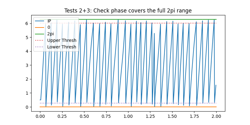
<matplotlib.legend.Legend object at 0x7f0eb98c3e90>
We can see that most cycles have instantaneous phase values crossing both the upper and lower threshold. Only the first and last cycles in these segments are missing these thresholds (as they are incomplete cycles cutt-off at the edges of this segment)
Finally, we check that we can detect a complete set of control points from
each cycle. The control points are the peak, trough, ascending zero-crossing
and descending zero-crossing. These can be computed from the IMF and a cycles
vector using emd.cycles.get_control_points
ctrl = emd.cycles.get_control_points(imf[:, 2], all_cycles[:, 2])

# Define some marker styles and legend labels for the control points.
markers = ['og', '^b', 'oc', 'vb', 'or']
label = ['Asc-Start', 'Peak', 'Desc', 'Trough', 'Asc-End']

# Plot the first 10 cycles with control points
ncycles = 20
start = 0

plt.figure()
plt.plot(111)
plt.title('Test 4: Control points')
for ii in range(ncycles):
    print('Cycle {0:2d} - {1}'.format(ii, ctrl[ii, :]))
    cycle = imf[all_cycles[:, 2] == ii, 2]
    plt.plot(np.arange(len(cycle))+start, cycle, 'k', label='Cycle')
    for jj in range(5):
        if np.isfinite(ctrl[ii, jj]):
            plt.plot(ctrl[ii, jj]+start, cycle[int(ctrl[ii, jj])], markers[jj], label=label[jj])
    start += len(cycle)

    # Only plot the legend for the first cycle
    if ii == 1:
        plt.legend()
plt.ylim(-400, 400)
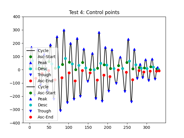
Cycle  0 - [0 5 8 13 16]
Cycle  1 - [0 4 7 11 15]
Cycle  2 - [0 4 8 12 16]
Cycle  3 - [0 3 7 12 15]
Cycle  4 - [0 4 8 13 17]
Cycle  5 - [0 4 8 13 17]
Cycle  6 - [0 3 7 12 15]
Cycle  7 - [0 4 8 12 17]
Cycle  8 - [0 3 8 13 19]
Cycle  9 - [0 5 9 14 17]
Cycle 10 - [0 4 8 12 16]
Cycle 11 - [0 3 7 12 15]
Cycle 12 - [0 4 9 15 20]
Cycle 13 - [0 4 10 16 20]
Cycle 14 - [0 4 7 12 15]
Cycle 15 - [0 3 7 11 15]
Cycle 16 - [0 2 5 9 12]
Cycle 17 - [0 3 7 11 15]
Cycle 18 - [0 4 7 11 15]
Cycle 19 - [0 2 4 nan 6]

(-400.0, 400.0)
Most of these cycles have the full set of control points present. Only ones
cycle (cycle-20 - close to the end) is missing an indicator for its
peak or trough. This is as a distortion in the cycle means that there are two
peaks and troughs present. In this case, get_control_points will return a
np.nan as the value for that peak.
We run these checks together automatically by setting the return_good
option to True. This is also the default option in the code. Here we run
cycle detection with the quality checks on and look at the first four seconds
of signal.
good_cycles = emd.cycles.get_cycle_vector(IP, return_good=True, phase_step=np.pi)

plt.figure(figsize=(10, 8))
plt.subplots_adjust(hspace=.3)
plt.subplot(311)
plt.plot(t[:sample_rate*4], imf[:sample_rate*4, 2], 'k')
plt.gca().set_xticklabels([])
plt.title('IMF-3')
plt.subplot(312)
plt.plot(t[:sample_rate*4], IP[:sample_rate*4, 2], 'b')
plt.gca().set_xticklabels([])
plt.plot((0, 4), (0, 0), label='0')
plt.plot((0, 4), (np.pi*2, np.pi*2), label='2pi')
plt.plot((0, 4), (np.pi*2-np.pi/12, np.pi*2-np.pi/12), ':', label='Upper Thresh')
plt.plot((0, 4), (np.pi/12, np.pi/12), ':', label='Lower Thresh')
plt.title('Instantanous Phase')
plt.ylabel('Radians')
plt.subplot(313)
plt.plot(t[:sample_rate*4], good_cycles[:sample_rate*4, 2])
plt.title('Good cycles')
plt.xlabel('Time (seconds)')
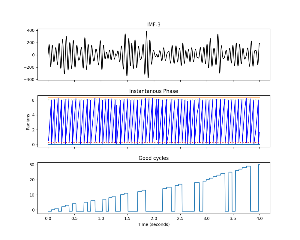
Text(0.5, 58.7222222222222, 'Time (seconds)')
Most cycles pass the checks but a few do fail. Closer inspection shows that these cycles tend to have large distortions or have very low amplitudes. Either way, the sift has not found a clear oscillation so these cycles should be interpreted with caution.
We can use the information in all_cycles to find explore the cycle
content of each IMF. For instance, this section prints the number of cycles
identified in each IMF
msg = 'IMF-{0} contains {1:3d} cycles of which {2:3d} ({3}%) are good'
for ii in range(all_cycles.shape[1]):
    all_count = all_cycles[:, ii].max()
    good_count = good_cycles[:, ii].max()
    percent = np.round(100*(good_count/all_count), 1)

    print(msg.format(ii+1, all_count, good_count, percent))
IMF-1 contains 116 cycles of which  14 (12.1%) are good
IMF-2 contains 348 cycles of which  20 (5.7%) are good
IMF-3 contains 150 cycles of which  70 (46.7%) are good
IMF-4 contains  99 cycles of which  77 (77.8%) are good
IMF-5 contains  44 cycles of which  38 (86.4%) are good
IMF-6 contains  20 cycles of which  18 (90.0%) are good
IMF-7 contains  11 cycles of which   9 (81.8%) are good
IMF-8 contains   5 cycles of which   3 (60.0%) are good
IMF-9 contains   2 cycles of which   0 (0.0%) are good
IMF-3 contains our simulated oscillation with a spectral peak around 15Hz. As we would expect, the cycle detection finds around 150 cycles in this 10 second segment. Many of these cycles pass our cycle-quality checks indicating that they have well behaved instantaneous phase profiles that can be interpreted in detail. Some cycles do not pass, indicating that parts of IMF-3 may not contain a strong oscillatory signal.
The lower frequency cycles (IMF 4+) have fewer and fewer cycles reflecting their slowing frequency content (each successive IMF extracts slower dynamics than the previous one). Again, most of these cycles pass the quality checks on their instantaneous phase. However, we also see that the the higher frequency IMFs 0 and 1 seem to contain fewer cycles than IMF-3. We would expect these IMFs to capture faster dynamics with more cycles in each IMF - so why are there fewer here?
The answer is in the quality of the instantaneous phase estimation in very fast oscillations. Lets plot the IMF and IP for IMF-1
plt.figure(figsize=(10, 8))
plt.subplots_adjust(hspace=.3)
plt.subplot(311)
plt.plot(t[:sample_rate//2], imf[:sample_rate//2, 0], 'k')
plt.gca().set_xticklabels([])
plt.title('IMF-0')

plt.subplot(312)
plt.plot(t[:sample_rate//2], IP[:sample_rate//2, 0], 'b')

plt.plot((0, .5), (0, 0), label='0')
plt.plot((0, .5), (np.pi*2, np.pi*2), label='2pi')
plt.plot((0, .5), (np.pi*2-np.pi/12, np.pi*2-np.pi/12), ':', label='Upper Thresh')
plt.plot((0, .5), (np.pi/12, np.pi/12), ':', label='Lower Thresh')

plt.gca().set_xticklabels([])
plt.title('Instantanous Phase')
plt.ylabel('Radians')

plt.subplot(313)
plt.plot(t[:sample_rate//2], good_cycles[:sample_rate//2, 0])
plt.title('Good cycles')
plt.xlabel('Time (seconds)')
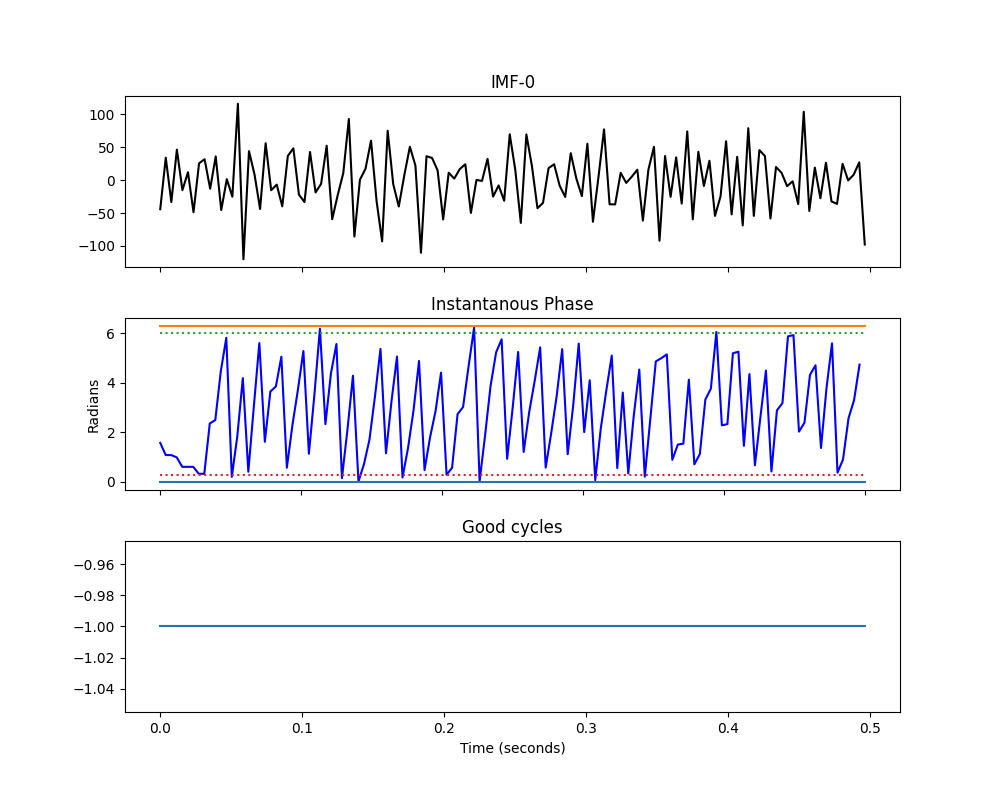
Text(0.5, 58.7222222222222, 'Time (seconds)')
The oscillations here are much faster than in IMF2. We only have a handful of samples for each potential cycle in IMF-1 compared to ~40 for IMF-3. As such, more cycles are showing distortions and failing the quality checks. In this case it is ok as there is no signal in IMF-1 in our simulation. Much of IMF-1 is noisy for this sift. We could potentially improve this by changing the sift parameters to compute more iterations for each IMF. This would increase the number of good cycles in IMF-1 but might lead to over-sifting in other IMFs. These parameters should be tuned for the priorities of each analysis.
Further Reading & References#
Andrew J. Quinn, Vítor Lopes-dos-Santos, Norden Huang, Wei-Kuang Liang, Chi-Hung Juan, Jia-Rong Yeh, Anna C. Nobre, David Dupret, and Mark W. Woolrich (2001) Within-cycle instantaneous frequency profiles report oscillatory waveform dynamics Journal of Neurophysiology 126:4, 1190-1208 https://doi.org/10.1152/jn.00201.2021
Total running time of the script: (0 minutes 1.851 seconds)