The Holospectrum

This tutorial shows how we can compute a holospectrum to characterise the distribution of power in a signal as a function of both frequency of the carrier wave and the frequency of any amplitude modulations

Simulating a signal with amplitude modulations

First of all, we import EMD alongside numpy and matplotlib. We will also use scipy’s ndimage module to smooth our results for visualisation later.

# sphinx_gallery_thumbnail_number = 5

import matplotlib.pyplot as plt
from scipy import ndimage
import numpy as np
import emd

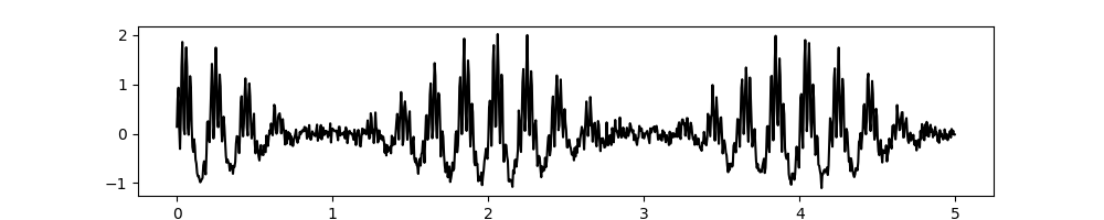
First we create a simulated signal to analyse. This signal will be composed of a linear trend and two oscillations, each with a different amplitude modulation.

seconds = 60
sample_rate = 200
t = np.linspace(0, seconds, seconds*sample_rate)

# First we create a slow 4.25Hz oscillation with a 0.5Hz amplitude modulation
slow = np.sin(2*np.pi*5*t) * (.5+(np.cos(2*np.pi*.5*t)/2))

# Second, we create a faster 37Hz oscillation that is amplitude modulated by the first.
fast = .5*np.sin(2*np.pi*37*t) * (slow+(.5+(np.cos(2*np.pi*.5*t)/2)))

# We create our signal by summing the oscillation and adding some noise
x = slow+fast + np.random.randn(*t.shape)*.1

# Plot the first 5 seconds of data
plt.figure(figsize=(10, 2))
plt.plot(t[:sample_rate*5], x[:sample_rate*5], 'k')

Out:

[<matplotlib.lines.Line2D object at 0x7f9d9c644f10>]

Next we run a simple sift with a cubic spline interpolation and estimate the instantaneous frequency statistics from it using the Normalised Hilbert Transform

config = emd.sift.get_config('mask_sift')
config['max_imfs'] = 7
config['mask_freqs'] = 50/sample_rate
config['mask_amp_mode'] = 'ratio_sig'
config['imf_opts/sd_thresh'] = 0.05
imf = emd.sift.mask_sift(x, **config)
IP, IF, IA = emd.spectra.frequency_transform(imf, sample_rate, 'nht')

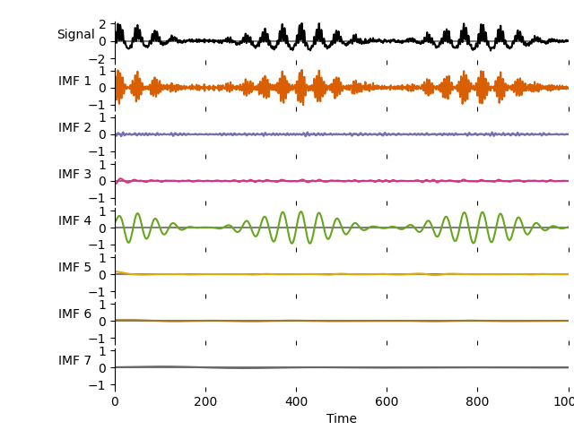
# Visualise the IMFs
emd.plotting.plot_imfs(imf[:sample_rate*5, :], cmap=True, scale_y=True)

Second-layer sift

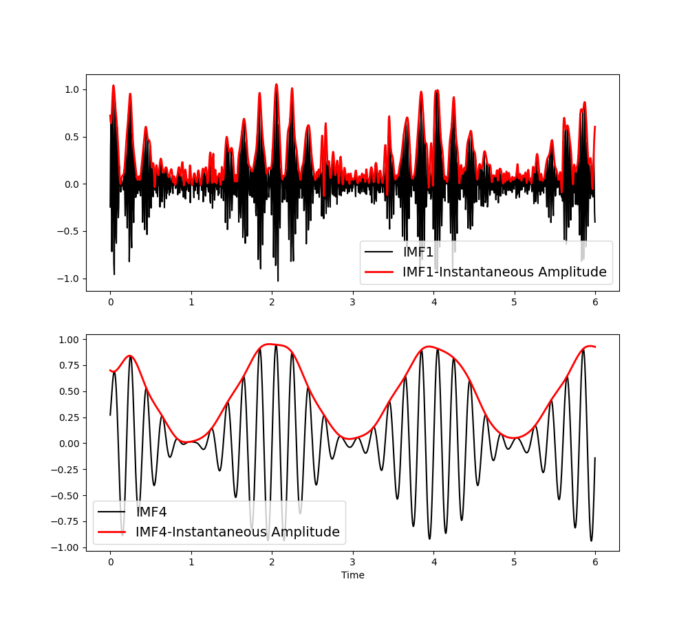
The first IMF contains the 30Hz oscillation and the fourth captures the 8Hz oscillation. Their amplitude modulations are described in the IA (Instantaneous Amplitude) variable. We can visualise these, note that the amplitude modulations (in red) are themselves oscillatory.

plt.figure(figsize=(10, 9))
plt.subplot(211)
plt.plot(t[:sample_rate*6], imf[:sample_rate*6, 0], 'k')
plt.plot(t[:sample_rate*6], IA[:sample_rate*6, 0], 'r', linewidth=2)
plt.legend(['IMF1', 'IMF1-Instantaneous Amplitude'], fontsize=14)
plt.subplot(212)
plt.plot(t[:sample_rate*6], imf[:sample_rate*6, 3], 'k')
plt.plot(t[:sample_rate*6], IA[:sample_rate*6, 3], 'r', linewidth=2)
plt.legend(['IMF4', 'IMF4-Instantaneous Amplitude'], fontsize=14)
plt.xlabel('Time')

Out:

Text(0.5, 69.7222222222222, 'Time')

We can describe the frequency content of these amplitude modulation signal with another EMD. This is called a second level sift which decomposes the instantaneous amplitude of each first level IMF with an additional set of IMFs.

# Helper function for the second level sift
def mask_sift_second_layer(IA, masks, config={}):
    imf2 = np.zeros((IA.shape[0], IA.shape[1], config['max_imfs']))
    for ii in range(IA.shape[1]):
        config['mask_freqs'] = masks[ii:]
        tmp = emd.sift.mask_sift(IA[:, ii], **config)
        imf2[:, ii, :tmp.shape[1]] = tmp
    return imf2


# Define sift parameters for the second level
masks = np.array([25/2**ii for ii in range(12)])/sample_rate
config = emd.sift.get_config('mask_sift')
config['mask_amp_mode'] = 'ratio_sig'
config['mask_amp'] = 2
config['max_imfs'] = 5
config['imf_opts/sd_thresh'] = 0.05
config['envelope_opts/interp_method'] = 'mono_pchip'

# Sift the first 5 first level IMFs
imf2 = emd.sift.mask_sift_second_layer(IA, masks, sift_args=config)

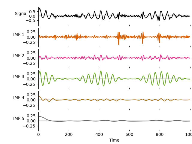
We can see that the oscillatory content in the amplitude modulations has been described with an additional set of IMFs. Here we plot the IMFs for the amplitude modulations of IMFs 1 (as plotted above).

emd.plotting.plot_imfs(imf2[:sample_rate*5, 0, :], scale_y=True, cmap=True)

The Holospectrum

We can compute the frequency stats for the second level IMFs using the same options as for the first levels.

IP2, IF2, IA2 = emd.spectra.frequency_transform(imf2, sample_rate, 'nht')

Finally, we want to visualise our results. We first define two sets of histogram bins, one for the main carrier frequency oscillations and one for the amplitude modulations.

# Carrier frequency histogram definition
carrier_hist = (1, 100, 128, 'log')
# AM frequency histogram definition
am_hist = (1e-2, 32, 64, 'log')

# Compute the 1d Hilbert-Huang transform (power over carrier frequency)
fcarrier, spec = emd.spectra.hilberthuang(IF, IA, carrier_hist, sum_imfs=False)

# Compute the 2d Hilbert-Huang transform (power over time x carrier frequency)
fcarrier, hht = emd.spectra.hilberthuang(IF, IA, carrier_hist, sum_time=False)
shht = ndimage.gaussian_filter(hht, 2)

# Compute the 3d Holospectrum transform (power over time x carrier frequency x AM frequency)
# Here we return the time averaged Holospectrum (power over carrier frequency x AM frequency)
fcarrier, fam, holo = emd.spectra.holospectrum(IF, IF2, IA2, carrier_hist, am_hist)
sholo = ndimage.gaussian_filter(holo, 1)

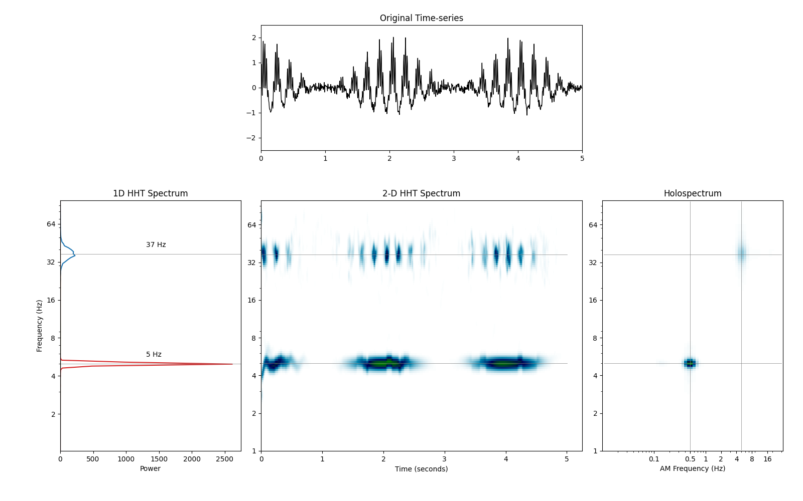
We summarise the results with a four part figure:

plt.figure(figsize=(16, 10))

# Plot a section of the time-course
plt.axes([.325, .7, .4, .25])
plt.plot(t[:sample_rate*5], x[:sample_rate*5], 'k', linewidth=1)
plt.xlim(0, 5)
plt.ylim(-2.5, 2.5)
plt.title('Original Time-series')

# Plot the 1d Hilbert-Huang Transform
plt.axes([.075, .1, .225, .5])
plt.plot(spec, fcarrier)
plt.plot((0, spec.max()*1.05), (5, 5), 'grey', linewidth=.5)
plt.text(spec.max()/2, 5.5, '5 Hz', verticalalignment='bottom')
plt.plot((0, spec.max()*1.05), (37, 37), 'grey', linewidth=.5)
plt.text(spec.max()/2, 41, '37 Hz', verticalalignment='bottom')
plt.title('1D HHT Spectrum')
plt.yscale('log')
plt.xlabel('Power')
plt.ylabel('Frequency (Hz)')
plt.yticks(2**np.arange(7), 2**np.arange(7))
plt.ylim(fcarrier[0], fcarrier[-1])
plt.xlim(0, spec.max()*1.05)

# Plot a section of the Hilbert-Huang transform
plt.axes([.325, .1, .4, .5])
plt.pcolormesh(t[:sample_rate*5], fcarrier, shht[:, :sample_rate*5], cmap='ocean_r', shading='nearest')
plt.yscale('log')
plt.plot((0, t[sample_rate*5]), (5, 5), 'grey', linewidth=.5)
plt.plot((0, t[sample_rate*5]), (37, 37), 'grey', linewidth=.5)
plt.title('2-D HHT Spectrum')
plt.xlabel('Time (seconds)')
plt.yticks(2**np.arange(7), 2**np.arange(7))

# Plot a the Holospectrum
plt.axes([.75, .1, .225, .5])
plt.pcolormesh(fam, fcarrier, sholo, cmap='ocean_r', shading='nearest')
plt.yscale('log')
plt.xscale('log')
plt.plot((fam[0], fam[-1]), (5, 5), 'grey', linewidth=.5)
plt.plot((fam[0], fam[-1]), (37, 37), 'grey', linewidth=.5)
plt.plot((.5, .5), (fcarrier[0], fcarrier[-1]), 'grey', linewidth=.5)
plt.plot((5, 5), (fcarrier[0], fcarrier[-1]), 'grey', linewidth=.5)
plt.title('Holospectrum')
plt.xlabel('AM Frequency (Hz)')
plt.yticks(2**np.arange(7), 2**np.arange(7))
plt.xticks([.1, .5, 1, 2, 4, 8, 16], [.1, .5, 1, 2, 4, 8, 16])

Out:

([<matplotlib.axis.XTick object at 0x7f9da4350d10>, <matplotlib.axis.XTick object at 0x7f9da4350a50>, <matplotlib.axis.XTick object at 0x7f9da4350690>, <matplotlib.axis.XTick object at 0x7f9da4333c10>, <matplotlib.axis.XTick object at 0x7f9da42ba110>, <matplotlib.axis.XTick object at 0x7f9da42ba490>, <matplotlib.axis.XTick object at 0x7f9da42bab90>], [Text(0.1, 0, '0.1'), Text(0.5, 0, '0.5'), Text(1.0, 0, '1'), Text(2.0, 0, '2'), Text(4.0, 0, '4'), Text(8.0, 0, '8'), Text(16.0, 0, '16')])

The four panels of the figure show: - top-center shows a segment of our original signal - bottom-leftshows the 1D Hilbert-Huang power spectrum - bottom-center shows a segment of the 2D Hilbert-Huang transform - bottom-right shows the Holospectrum summed over the time dimension

We can see prominent peaks at 5Hz and at 37Hz in the 1D Hilbert-Huang spectrum. The 2D Hilbert-Huang spectrum extends this over time showing fluctuations in both of these oscillations. Finall, the Holospectrum reveals that these fluctuations in power are themselves oscillating. The 5Hz rhythm has ampltude modulations of 0.5Hz and the 37Hz rhythm has ampltiude modulations of 5Hz.

Finally we can quantify the phase-amplitude coupling in our signal. We do this by splitting the phase of the 5Hz signal into bins and computing the average of the 2D Hilbert-Huang spectrum for each bin. This is implemented in the emd.cycles.bin_by_phase function.

hht_by_phase, _, _ = emd.cycles.bin_by_phase(IP[:, 3], hht.T)

plt.figure(figsize=(8, 8))
plt.subplot(121)
plt.pcolormesh(fam, fcarrier, sholo, cmap='ocean_r', shading='nearest')
plt.yscale('log')
plt.xscale('log')
plt.title('Holospectrum')
plt.xlabel('AM Frequency (Hz)')
plt.ylabel('Frequency (Hz)')
plt.yticks(2**np.arange(7), 2**np.arange(7))
plt.xticks([.1, .5, 1, 2, 4, 8, 16], [.1, .5, 1, 2, 4, 8, 16])

plt.subplot(122)
plt.pcolormesh(np.linspace(-np.pi, np.pi, 24), fcarrier, hht_by_phase.T, cmap='ocean_r', shading='auto')
plt.yscale('log')
plt.yticks(2**np.arange(7), 2**np.arange(7))
plt.xticks(np.linspace(-np.pi, np.pi, 5), ['Asc', 'Peak', 'Desc', 'Trough', 'Asc'])
plt.xlabel('Theta Phase')
plt.colorbar()
plt.title('HHT by 5Hz Phase')

Out:

Text(0.5, 1.0, 'HHT by 5Hz Phase')

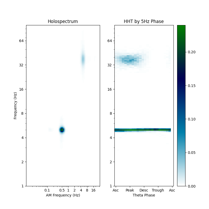
The summary figure shows the Holospectrum alongside the power in the HHT across phase bins with carrier frequency in the y-axis and phase in the x-axis. This plot is sometime known as a comodulogram. We see that power in the 37Hz oscillation peaks around the peak of the 5Hz cycle confirming the presence of phase-ampltiude coupling between these two signals.

The 5Hz power is visible as a flat line across all phase. This indicates that neither the power or the frequency of this signal is changing within the cycle.

previous

The Hilbert-Huang Transform

next

Cross-Frequency Coupling