Cross-Frequency Coupling

The spectrum tools in EMD can be used to explore cross-frequency interactions in oscillatory signals. The simplest approach is to look at how the phase, frequency or amplitude of a high-frequency signal interacts with the phase of a low frequency signal. This can be extended into 2 or 3 dimensions by exploring the relationship between low-frequency phase and the Hilbert-Huang Transform and Holospectrum. This tutorial shows some examples of these analyses with three signals with varying phase-amplitude coupling profiles.

Simulating a signal with amplitude modulations

First of all, we import EMD alongside numpy and matplotlib. We will also use scipy’s ndimage module to smooth our results for visualisation later.

# sphinx_gallery_thumbnail_number = 8

import matplotlib.pyplot as plt
import numpy as np
import emd

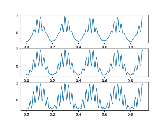
Next, we create three simulated signal to analyse. Each signal will be composed of two oscillations - a low-frequency signal at 5Hz and a high-frequency signal at 37Hz. The three variants of this signal differ in how the amplitude of the high frequency signal varies with the phase of the low frequency signal. We vary the width of the high-frequency burst across the three signals.

seconds = 60
sample_rate = 200
t = np.linspace(0, seconds, seconds*sample_rate)

# First we create a slow 5Hz oscillation and a fast 37Hz oscillation
slow = np.sin(2*np.pi*5*t - np.pi/2)
fast = np.cos(2*np.pi*37*t)

# Next we create three different amplitude modulation signals for the fast
# oscillation. One sinusoidal, one wide modulation and one narrow modulation.
# These cases differ by the duration of the high frequency burst.

fast_am = 0.5*slow + 0.5
fast_am_narrow = fast_am**3
fast_am_wide = 1 - (0.5*-slow + 0.5)**3

# We create our signal by summing the oscillation and adding some noise
x = slow + fast * fast_am + np.random.randn(*t.shape) * .05
x_wide = slow + fast * fast_am_wide + np.random.randn(*t.shape) * .05
x_narrow = slow + fast * fast_am_narrow + np.random.randn(*t.shape) * .05

Let’s take a look at the three signals.

plt.figure()
plt.subplot(311)
plt.plot(t[:seconds*3], x_narrow[:seconds*3])
plt.subplot(312)
plt.plot(t[:seconds*3], x[:seconds*3])
plt.subplot(313)
plt.plot(t[:seconds*3], x_wide[:seconds*3])

Out:

[<matplotlib.lines.Line2D object at 0x7f9d9cd8c910>]

The narrow amplitude modulated signal is plotted on the top, the sinusoidally modulated case in the middle and the wide amplitude modulation on the bottom. All three high-frequency signals peak at the same point in the low-frequency cycle.

Next we run a mask sift on these signals to create IMFs for each case before running the frequency transforms to get the instantaneous phase, frequency and phase.

# Define a mask sift config
config = emd.sift.get_config('mask_sift')
config['max_imfs'] = 7
config['mask_freqs'] = 50/sample_rate
config['mask_amp_mode'] = 'ratio_sig'
config['imf_opts/sd_thresh'] = 0.05
config['extrema_opts/method'] = 'rilling'

imf = emd.sift.mask_sift(x, **config)
IP, IF, IA = emd.spectra.frequency_transform(imf, sample_rate, 'hilbert')

imf_wide = emd.sift.mask_sift(x_wide, **config)
IP_wide, IF_wide, IA_wide = emd.spectra.frequency_transform(imf_wide, sample_rate, 'hilbert')

imf_narrow = emd.sift.mask_sift(x_narrow, **config)
IP_narrow, IF_narrow, IA_narrow = emd.spectra.frequency_transform(imf_narrow, sample_rate, 'hilbert')

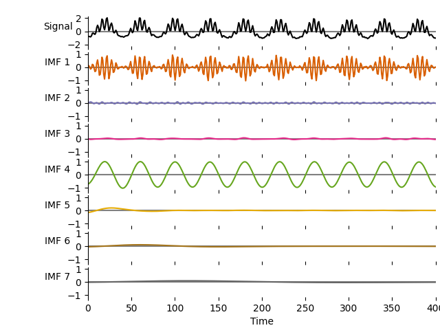
We plot up the IMFs for the sinusoidally modulated case and see that the fast signal is isolated into the first IMF and the low-frequency signal is in the fourth. The rest of the IMFs largely contain noise

emd.plotting.plot_imfs(imf[:sample_rate*2, :], cmap=True, scale_y=True)

1D Phase-amplitude coupling with instantaneous amplitude

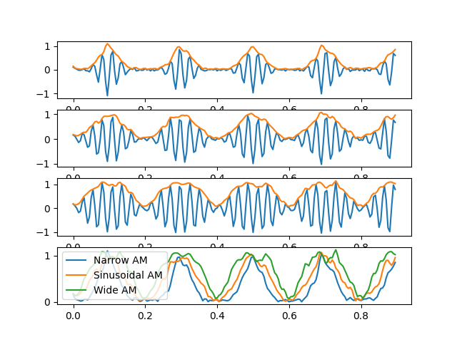
Let’s zoom in on the fast signals containing the simulated amplitude modulations. Here, we plot the first IMF for each of the three signals with different modulation widths.

plt.figure()
plt.subplot(411)
plt.plot(t[:seconds*3], imf_narrow[:seconds*3, 0])
plt.plot(t[:seconds*3], IA_narrow[:seconds*3, 0])
plt.subplot(412)
plt.plot(t[:seconds*3], imf[:seconds*3, 0])
plt.plot(t[:seconds*3], IA[:seconds*3, 0])
plt.subplot(413)
plt.plot(t[:seconds*3], imf_wide[:seconds*3, 0])
plt.plot(t[:seconds*3], IA_wide[:seconds*3, 0])
plt.subplot(414)
plt.plot(t[:seconds*3], IA_narrow[:seconds*3, 0])
plt.plot(t[:seconds*3], IA[:seconds*3, 0])
plt.plot(t[:seconds*3], IA_wide[:seconds*3, 0])
plt.legend(['Narrow AM', 'Sinusoidal AM', 'Wide AM'])

Out:

<matplotlib.legend.Legend object at 0x7f9d9c65ba90>

The narrow modulation is on top-row, the sinusoidal modulation in the second and the wide modulation is in the third. All three amplitude modulations on top of each other in the bottom row. By eye, the different modulation widths are clear but it is perhaps less obvious how we can quantify this effect.

One simple approach is to explore how the instantaneous amplitude of each case varies with the phase of the low-frequency signal component. We can compute this with emd.cycles.bin_by_phase. The inputs take a phase signal which is segmented into a set of time-bins in which the second input is averaged. (A very similar alternative analysis could be run using emd.cycles.phase_align).

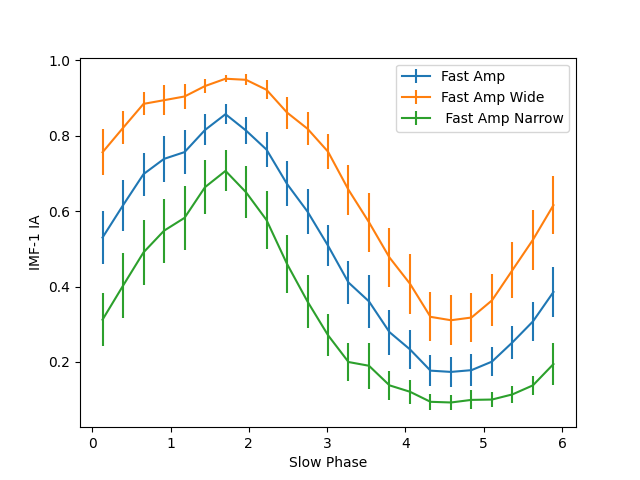
We compute the average high-frequency IA as a function of low-frequency phase for each of our three examples and plot the result:

ia_by_phase, ia_by_phase_var, phase_bins = emd.cycles.bin_by_phase(IP[:, 4], IA[:, 0], nbins=24)
ia_by_phase_wide, ia_by_phase_wide_var, _ = emd.cycles.bin_by_phase(IP[:, 4], IA_wide[:, 0], nbins=24)
ia_by_phase_narrow, ia_by_phase_narrow_var, _ = emd.cycles.bin_by_phase(IP[:, 4], IA_narrow[:, 0], nbins=24)

plt.figure()
plt.errorbar(phase_bins, ia_by_phase, yerr=ia_by_phase_var)
plt.errorbar(phase_bins, ia_by_phase_wide, yerr=ia_by_phase_wide_var)
plt.errorbar(phase_bins, ia_by_phase_narrow, yerr=ia_by_phase_narrow_var)
plt.legend(['Fast Amp', 'Fast Amp Wide', ' Fast Amp Narrow'])
plt.xlabel('Slow Phase')
plt.ylabel('IMF-1 IA')

Out:

Text(42.722222222222214, 0.5, 'IMF-1 IA')

Now, we see the three amplitude modulation profiles directly linked to theta phase - there is a clear peak in high-frequency amplitude at one point in theta phase confirming the presence of phase-amplitude coupling in this signal. We can also see the different in modulation width in the three signals.

2D Phase-amplitude coupling with the HHT

We can run a two-dimensional equivalent to the above analysis by exploring how a whole Hilbert-Huang transform varies across low-frequency phase. This gives us a bit more information than our first analysis. Specifically we can also see which frequency the amplitude modulated signal is peaking at.

The first step is to compute the Hilbert-Huang Transform (HHT) for our three signals.

freq_edges, freq_centres = emd.spectra.define_hist_bins(10, 75, 75, 'log')

f, hht = emd.spectra.hilberthuang(IF, IA, freq_edges, mode='amplitude', sum_time=False)
f, hht_wide = emd.spectra.hilberthuang(IF_wide, IA_wide, freq_edges, mode='amplitude', sum_time=False)
f, hht_narrow = emd.spectra.hilberthuang(IF_narrow, IA_narrow, freq_edges, mode='amplitude', sum_time=False)

Out:

[10.         10.27229501 10.55200448 10.8393303  11.13447986 11.43766619
 11.74910814 12.06903049 12.39766417 12.73524639 13.08202079 13.4382377
 13.80415421 14.18003444 14.56614971 14.9627787  15.3702077  15.78873079
 16.21865005 16.66027581 17.11392681 17.5799305  18.05862324 18.55035054
 19.05546733 19.57433821 20.10733767 20.65485045 21.21727173 21.79500745
 22.38847463 22.99810163 23.62432847 24.26760715 24.92840199 25.60718994
 26.30446095 27.02071831 27.75647899 28.51227407 29.28864907 30.08616438
 30.90539563 31.74693414 32.61138732 33.49937913 34.41155052 35.34855988
 36.31108353 37.29981623 38.31547162 39.3587828  40.43050283 41.53140526
 42.66228471 43.82395744 45.01726195 46.24305954 47.50223498 48.79569715
 50.12437965 51.48924151 52.89126787 54.33147072 55.81088957 57.33059225
 58.89167569 60.49526664 62.14252258 63.83463248 65.57281768 67.3583328
 69.19246661 71.07654297 73.01192178 75.        ]
[10.         10.27229501 10.55200448 10.8393303  11.13447986 11.43766619
 11.74910814 12.06903049 12.39766417 12.73524639 13.08202079 13.4382377
 13.80415421 14.18003444 14.56614971 14.9627787  15.3702077  15.78873079
 16.21865005 16.66027581 17.11392681 17.5799305  18.05862324 18.55035054
 19.05546733 19.57433821 20.10733767 20.65485045 21.21727173 21.79500745
 22.38847463 22.99810163 23.62432847 24.26760715 24.92840199 25.60718994
 26.30446095 27.02071831 27.75647899 28.51227407 29.28864907 30.08616438
 30.90539563 31.74693414 32.61138732 33.49937913 34.41155052 35.34855988
 36.31108353 37.29981623 38.31547162 39.3587828  40.43050283 41.53140526
 42.66228471 43.82395744 45.01726195 46.24305954 47.50223498 48.79569715
 50.12437965 51.48924151 52.89126787 54.33147072 55.81088957 57.33059225
 58.89167569 60.49526664 62.14252258 63.83463248 65.57281768 67.3583328
 69.19246661 71.07654297 73.01192178 75.        ]
[10.         10.27229501 10.55200448 10.8393303  11.13447986 11.43766619
 11.74910814 12.06903049 12.39766417 12.73524639 13.08202079 13.4382377
 13.80415421 14.18003444 14.56614971 14.9627787  15.3702077  15.78873079
 16.21865005 16.66027581 17.11392681 17.5799305  18.05862324 18.55035054
 19.05546733 19.57433821 20.10733767 20.65485045 21.21727173 21.79500745
 22.38847463 22.99810163 23.62432847 24.26760715 24.92840199 25.60718994
 26.30446095 27.02071831 27.75647899 28.51227407 29.28864907 30.08616438
 30.90539563 31.74693414 32.61138732 33.49937913 34.41155052 35.34855988
 36.31108353 37.29981623 38.31547162 39.3587828  40.43050283 41.53140526
 42.66228471 43.82395744 45.01726195 46.24305954 47.50223498 48.79569715
 50.12437965 51.48924151 52.89126787 54.33147072 55.81088957 57.33059225
 58.89167569 60.49526664 62.14252258 63.83463248 65.57281768 67.3583328
 69.19246661 71.07654297 73.01192178 75.        ]

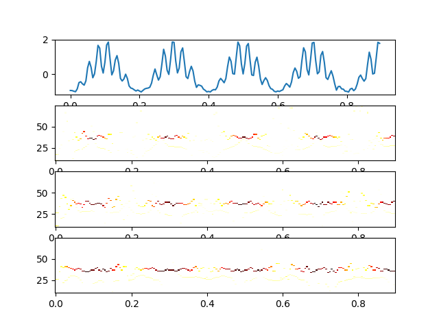
A quick summary figure shows us the HHT representation of our amplitude modulated signals. The recurring high-frequency bursts are visible in all three cases with the duration of each burst differing between the narrow, sinusoidal and widde cases.

plt.figure()
plt.subplot(411)
plt.plot(t[:seconds*3], x[:seconds*3])
plt.subplot(412)
plt.pcolormesh(t[:seconds*3], f, hht_narrow[:, :seconds*3], cmap='hot_r', shading='auto')
plt.subplot(413)
plt.pcolormesh(t[:seconds*3], f, hht[:, :seconds*3], cmap='hot_r', shading='auto')
plt.subplot(414)
plt.pcolormesh(t[:seconds*3], f, hht_wide[:, :seconds*3], cmap='hot_r', shading='auto')

Out:

<matplotlib.collections.QuadMesh object at 0x7f9da4178dd0>

We can use emd.cycles.bin_by_phase to explore how high dimensional signals vary with a phase time-course - as long as the first dimension of the signal to be averaged matches the length of the phase signal. Here, we bin the HHT by low-frequency phase for each of our three signals.

hht_by_phase, _, phase_centres = emd.cycles.bin_by_phase(IP[:, 4], hht.T)
hht_by_phase_wide, _, _ = emd.cycles.bin_by_phase(IP[:, 4], hht_wide.T)
hht_by_phase_narrow, _, _ = emd.cycles.bin_by_phase(IP[:, 4], hht_narrow.T)

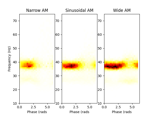
Let’s make a quick summary figure of the phase-resolved HHTs.

plt.figure()
plt.subplot(131)
plt.pcolormesh(phase_centres, freq_centres, hht_by_phase_narrow.T, vmax=0.25, cmap='hot_r', shading='auto')
plt.xlabel('Phase (rads')
plt.ylabel('Frequency (Hz)')
plt.title('Narrow AM')
plt.subplot(132)
plt.pcolormesh(phase_centres, freq_centres, hht_by_phase.T, vmax=0.25, cmap='hot_r', shading='auto')
plt.xlabel('Phase (rads')
plt.title('Sinusoidal AM')
plt.subplot(133)
plt.pcolormesh(phase_centres, freq_centres, hht_by_phase_wide.T, vmax=0.25, cmap='hot_r', shading='auto')
plt.xlabel('Phase (rads')
plt.title('Wide AM')

Out:

Text(0.5, 1.0, 'Wide AM')

We can see that all three cases peak around the same point in phase (around pi/2) at at the same frequency (37Hz) but clearly differ in their modulation width. Though this is visible here, we still don’t directly quantify this feature with the Hilbert-Huang Transform.

We can quantify this difference by looking at the frequency content of the high-frequency signal amplitude envelopes. It appears like the signal with wide modulation has a lower frequency amplitude modulation How can we measure this?

Quantifying the frequency of amplitude modulations

The Holospectrum provides a method for direct quantification of the frequency and timing of amplitude modulations in oscillatory signal. The concept and method for Holospectrum estimation are covered in detail in the previous tutorial - here we will only cover its application in cross-frequency coupling.

First, we compute the second-layer sift of our amplitude modulated signals. We apply a mask-sift at the second level to the instantaneous amplitude of our high frequency signals. The frequency transform of the resulting second-layer IMFs is then computed using the Hilbert transform.

# Reduce the mask frequencies for the second layer sift - otherwise we use the
# same config as the first layer.
config['mask_freqs'] = [10/sample_rate/ii for ii in range(1, 10)]


imf2 = emd.sift.mask_sift_second_layer(IA[:, 0], config['mask_freqs'], sift_args=config)
IP2, IF2, IA2 = emd.spectra.frequency_transform(imf2, sample_rate, 'hilbert')

imf2_wide = emd.sift.mask_sift_second_layer(IA_wide[:, 0], config['mask_freqs'], sift_args=config)
IP2_wide, IF2_wide, IA2_wide = emd.spectra.frequency_transform(imf2_wide, sample_rate, 'hilbert')

imf2_narrow = emd.sift.mask_sift_second_layer(IA_narrow[:, 0], config['mask_freqs'], sift_args=config)
IP2_narrow, IF2_narrow, IA2_narrow = emd.spectra.frequency_transform(imf2_narrow, sample_rate, 'hilbert')

Next we compute the Holospectrum itself. We define a two sets of frequency bins for the first layer oscillations and second layer amplitude modulations before computing the Holospectrum using emd.spectra.holospectrum.

freq_edges, freq_centres = emd.spectra.define_hist_bins(1, 75, 75, 'log')
freq_edges_low, freq_centres_low = emd.spectra.define_hist_bins(2, 10, 20, 'linear')

fcarrier, fam, holo = emd.spectra.holospectrum(IF[:, 0, None], IF2, IA2, freq_edges, freq_edges_low)
fcarrier, fam, holo_narrow = emd.spectra.holospectrum(IF_narrow[:, 0, None], IF2_narrow, IA2_narrow, freq_edges, freq_edges_low)
fcarrier, fam, holo_wide = emd.spectra.holospectrum(IF_wide[:, 0, None], IF2_wide, IA2_wide, freq_edges, freq_edges_low)

# Holo is [second-layer frequencies x first-layer frequencies]
print(holo.shape)

Out:

[ 1.          1.05925572  1.12202268  1.18850893  1.25893488  1.33353397
  1.41255349  1.49625536  1.58491704  1.67883244  1.77831286  1.88368806
  1.99530735  2.11354072  2.23878009  2.37144061  2.51196202  2.66081014
  2.81847835  2.98548931  3.16239662  3.3497867   3.54828071  3.75853663
  3.98125142  4.21716333  4.46705437  4.73175288  5.01213629  5.30913402
  5.62373057  5.95696876  6.30995321  6.68385402  7.07991058  7.49943576
  7.94382021  8.41453698  8.9131464   9.44130129 10.00075237 10.59335413
 11.22107093 11.88598354 12.59029602 13.33634304 14.12659762 14.96367929
 15.85036285 16.78958747 17.78446652 18.83829785 19.9545747  21.13699734
 22.38948529 23.7161903  25.12151017 26.61010328 28.18690404 29.85713927
 31.62634548 33.50038727 35.48547675 37.58819414 39.81550955 42.17480613
 44.67390453 47.3210888  50.12513387 53.09533464 56.24153679 59.5741694
 63.10427955 66.84356891 70.80443255 75.        ]
[ 2.   2.4  2.8  3.2  3.6  4.   4.4  4.8  5.2  5.6  6.   6.4  6.8  7.2
  7.6  8.   8.4  8.8  9.2  9.6 10. ]
[ 1.          1.05925572  1.12202268  1.18850893  1.25893488  1.33353397
  1.41255349  1.49625536  1.58491704  1.67883244  1.77831286  1.88368806
  1.99530735  2.11354072  2.23878009  2.37144061  2.51196202  2.66081014
  2.81847835  2.98548931  3.16239662  3.3497867   3.54828071  3.75853663
  3.98125142  4.21716333  4.46705437  4.73175288  5.01213629  5.30913402
  5.62373057  5.95696876  6.30995321  6.68385402  7.07991058  7.49943576
  7.94382021  8.41453698  8.9131464   9.44130129 10.00075237 10.59335413
 11.22107093 11.88598354 12.59029602 13.33634304 14.12659762 14.96367929
 15.85036285 16.78958747 17.78446652 18.83829785 19.9545747  21.13699734
 22.38948529 23.7161903  25.12151017 26.61010328 28.18690404 29.85713927
 31.62634548 33.50038727 35.48547675 37.58819414 39.81550955 42.17480613
 44.67390453 47.3210888  50.12513387 53.09533464 56.24153679 59.5741694
 63.10427955 66.84356891 70.80443255 75.        ]
[ 2.   2.4  2.8  3.2  3.6  4.   4.4  4.8  5.2  5.6  6.   6.4  6.8  7.2
  7.6  8.   8.4  8.8  9.2  9.6 10. ]
[ 1.          1.05925572  1.12202268  1.18850893  1.25893488  1.33353397
  1.41255349  1.49625536  1.58491704  1.67883244  1.77831286  1.88368806
  1.99530735  2.11354072  2.23878009  2.37144061  2.51196202  2.66081014
  2.81847835  2.98548931  3.16239662  3.3497867   3.54828071  3.75853663
  3.98125142  4.21716333  4.46705437  4.73175288  5.01213629  5.30913402
  5.62373057  5.95696876  6.30995321  6.68385402  7.07991058  7.49943576
  7.94382021  8.41453698  8.9131464   9.44130129 10.00075237 10.59335413
 11.22107093 11.88598354 12.59029602 13.33634304 14.12659762 14.96367929
 15.85036285 16.78958747 17.78446652 18.83829785 19.9545747  21.13699734
 22.38948529 23.7161903  25.12151017 26.61010328 28.18690404 29.85713927
 31.62634548 33.50038727 35.48547675 37.58819414 39.81550955 42.17480613
 44.67390453 47.3210888  50.12513387 53.09533464 56.24153679 59.5741694
 63.10427955 66.84356891 70.80443255 75.        ]
[ 2.   2.4  2.8  3.2  3.6  4.   4.4  4.8  5.2  5.6  6.   6.4  6.8  7.2
  7.6  8.   8.4  8.8  9.2  9.6 10. ]
(75, 20)

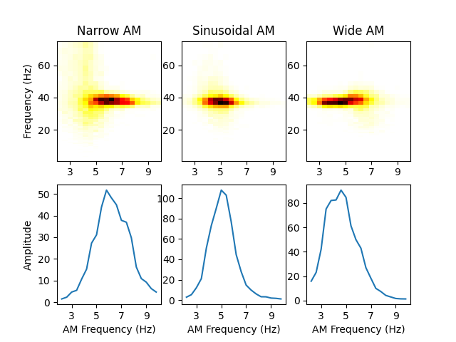
The output holospectrum is a 2d matrix of first-layer frequencies by second-layer frequencies (we sum across time dimension by default). We next make a summary plot with this 2d Holospectrum for each case in the top row and the average holospectrum across first-layer frequencies (ie expressing the energy in signals with given amplitude modulation frequencies across all first-layer frequencies.)

plt.figure()
plt.subplot(231)
plt.pcolormesh(freq_centres_low, freq_centres, holo_narrow, cmap='hot_r', shading='auto')
plt.ylabel('Frequency (Hz)')
plt.xticks(np.arange(3, 10, 2))
plt.title('Narrow AM')
plt.subplot(234)
plt.plot(freq_centres_low, holo_narrow[62, :])
plt.xlabel('AM Frequency (Hz)')
plt.xticks(np.arange(3, 10, 2))
plt.ylabel('Amplitude')

plt.subplot(232)
plt.pcolormesh(freq_centres_low, freq_centres, holo, cmap='hot_r', shading='auto')
plt.xticks(np.arange(3, 10, 2))
plt.title('Sinusoidal AM')
plt.subplot(235)
plt.plot(freq_centres_low, holo[62, :])
plt.xticks(np.arange(3, 10, 2))
plt.xlabel('AM Frequency (Hz)')

plt.subplot(233)
plt.pcolormesh(freq_centres_low, freq_centres, holo_wide, cmap='hot_r', shading='auto')
plt.xticks(np.arange(3, 10, 2))
plt.title('Wide AM')
plt.subplot(236)
plt.plot(freq_centres_low, holo_wide[62, :])
plt.xticks(np.arange(3, 10, 2))
plt.xlabel('AM Frequency (Hz)')

Out:

Text(0.5, 23.52222222222222, 'AM Frequency (Hz)')

The holospectra on the top row show the distribution of energy across frequency and amplitude modulation frequency within each signal. The bottom row sums the holospectra across the y-axis to summarise just the distribution of energy across apmlitude modulation frequencies.

The sinusoidal signal has a clear peak with a frequency of 37Hz with amplitude modulations of 5Hz - exactly as we would expect from this simulation. The other signals have a similar peak but slightly skewed to higher or lower amplitude modulation frequencies. The signal with narrow modulation has higher amplitude modulation frequencies - reflecting the faster/sharper amplitude modulation profile of the signal. In contrast, the signal with wide amplitude modulations skews towards slower amplitude modulations - reflectings its slower, flatter amplitude modulation profile.

The holospectrum provides a convenient summary of the amplitude modulations in a signal, but doesn’t explicitly link them to the phase of a lower frequency signal. To complete a full cross-frequency coupling analysis with the Holospectrum we need to show not only that our high frequency signal has amplitude modulations but that those amplitude modulations are specifically linked to a n observed low-frequency signal.

3D phase-amplitude coupling with the Holospectrum

We can link the Holospectrum to low frequency phase in exactly the same way as we analysed the instantaneous amplitude and Hilbert-Huang Transforms. First, we have to recompute the holospectra whilst preserving the time dimension in the output. By default, the holospectrum is summed over time before being returned - we can ask for the full 3D holospectrum to be returned by setting squash_time=False in the emd.spectra.holospectrum call.

# Define a new set of second-layer frequencies - slightly wider than the last one.
freq_edges_low, freq_centres_low = emd.spectra.define_hist_bins(.5, 15, 32, 'linear')

fcarrier, fam, holot = emd.spectra.holospectrum(IF[:, 0, None], IF2, IA2,
                                 freq_edges, freq_edges_low, sum_time=False)
fcarrier, fam, holot_wide = emd.spectra.holospectrum(IF_wide[:, 0, None], IF2_wide, IA2_wide,
                                      freq_edges, freq_edges_low, sum_time=False)
fcarrier, fam, holot_narrow = emd.spectra.holospectrum(IF_narrow[:, 0, None], IF2_narrow, IA2_narrow,
                                        freq_edges, freq_edges_low, sum_time=False)


# holot is [second-layer frequencies x first-layer frequencies x time samples]
print(holot.shape)

Out:

[ 1.          1.05925572  1.12202268  1.18850893  1.25893488  1.33353397
  1.41255349  1.49625536  1.58491704  1.67883244  1.77831286  1.88368806
  1.99530735  2.11354072  2.23878009  2.37144061  2.51196202  2.66081014
  2.81847835  2.98548931  3.16239662  3.3497867   3.54828071  3.75853663
  3.98125142  4.21716333  4.46705437  4.73175288  5.01213629  5.30913402
  5.62373057  5.95696876  6.30995321  6.68385402  7.07991058  7.49943576
  7.94382021  8.41453698  8.9131464   9.44130129 10.00075237 10.59335413
 11.22107093 11.88598354 12.59029602 13.33634304 14.12659762 14.96367929
 15.85036285 16.78958747 17.78446652 18.83829785 19.9545747  21.13699734
 22.38948529 23.7161903  25.12151017 26.61010328 28.18690404 29.85713927
 31.62634548 33.50038727 35.48547675 37.58819414 39.81550955 42.17480613
 44.67390453 47.3210888  50.12513387 53.09533464 56.24153679 59.5741694
 63.10427955 66.84356891 70.80443255 75.        ]
[ 0.5       0.953125  1.40625   1.859375  2.3125    2.765625  3.21875
  3.671875  4.125     4.578125  5.03125   5.484375  5.9375    6.390625
  6.84375   7.296875  7.75      8.203125  8.65625   9.109375  9.5625
 10.015625 10.46875  10.921875 11.375    11.828125 12.28125  12.734375
 13.1875   13.640625 14.09375  14.546875 15.      ]
[ 1.          1.05925572  1.12202268  1.18850893  1.25893488  1.33353397
  1.41255349  1.49625536  1.58491704  1.67883244  1.77831286  1.88368806
  1.99530735  2.11354072  2.23878009  2.37144061  2.51196202  2.66081014
  2.81847835  2.98548931  3.16239662  3.3497867   3.54828071  3.75853663
  3.98125142  4.21716333  4.46705437  4.73175288  5.01213629  5.30913402
  5.62373057  5.95696876  6.30995321  6.68385402  7.07991058  7.49943576
  7.94382021  8.41453698  8.9131464   9.44130129 10.00075237 10.59335413
 11.22107093 11.88598354 12.59029602 13.33634304 14.12659762 14.96367929
 15.85036285 16.78958747 17.78446652 18.83829785 19.9545747  21.13699734
 22.38948529 23.7161903  25.12151017 26.61010328 28.18690404 29.85713927
 31.62634548 33.50038727 35.48547675 37.58819414 39.81550955 42.17480613
 44.67390453 47.3210888  50.12513387 53.09533464 56.24153679 59.5741694
 63.10427955 66.84356891 70.80443255 75.        ]
[ 0.5       0.953125  1.40625   1.859375  2.3125    2.765625  3.21875
  3.671875  4.125     4.578125  5.03125   5.484375  5.9375    6.390625
  6.84375   7.296875  7.75      8.203125  8.65625   9.109375  9.5625
 10.015625 10.46875  10.921875 11.375    11.828125 12.28125  12.734375
 13.1875   13.640625 14.09375  14.546875 15.      ]
[ 1.          1.05925572  1.12202268  1.18850893  1.25893488  1.33353397
  1.41255349  1.49625536  1.58491704  1.67883244  1.77831286  1.88368806
  1.99530735  2.11354072  2.23878009  2.37144061  2.51196202  2.66081014
  2.81847835  2.98548931  3.16239662  3.3497867   3.54828071  3.75853663
  3.98125142  4.21716333  4.46705437  4.73175288  5.01213629  5.30913402
  5.62373057  5.95696876  6.30995321  6.68385402  7.07991058  7.49943576
  7.94382021  8.41453698  8.9131464   9.44130129 10.00075237 10.59335413
 11.22107093 11.88598354 12.59029602 13.33634304 14.12659762 14.96367929
 15.85036285 16.78958747 17.78446652 18.83829785 19.9545747  21.13699734
 22.38948529 23.7161903  25.12151017 26.61010328 28.18690404 29.85713927
 31.62634548 33.50038727 35.48547675 37.58819414 39.81550955 42.17480613
 44.67390453 47.3210888  50.12513387 53.09533464 56.24153679 59.5741694
 63.10427955 66.84356891 70.80443255 75.        ]
[ 0.5       0.953125  1.40625   1.859375  2.3125    2.765625  3.21875
  3.671875  4.125     4.578125  5.03125   5.484375  5.9375    6.390625
  6.84375   7.296875  7.75      8.203125  8.65625   9.109375  9.5625
 10.015625 10.46875  10.921875 11.375    11.828125 12.28125  12.734375
 13.1875   13.640625 14.09375  14.546875 15.      ]
(75, 32, 12000)

Now that we have a time-varying holospectrum estimate - we can compute its average in different low-frequency bins by using emd.cycles.bin_by_phase as for our previous analyses.

holo_by_phase, _, phase_bins = emd.cycles.bin_by_phase(IP[:, 4], np.swapaxes(holot, 0, 2))
holo_by_phase_wide, _, _ = emd.cycles.bin_by_phase(IP[:, 4], np.swapaxes(holot_wide, 0, 2))
holo_by_phase_narrow, _, _ = emd.cycles.bin_by_phase(IP[:, 4], np.swapaxes(holot_narrow, 0, 2))

# holo_by_phase is [phase bins x second-layer frequencies x first-layer frequencies]
print(holo_by_phase.shape)

Out:

(24, 32, 75)

holo_by_phase now contains a summary of the energy in each signal separated by first-layer frequencies, second layer-frequencies and by the phase of our low frequency signal. If the amplitude modulations we observed in our signals are explicitly linked to the 5Hz phase - we should be able to see it here.

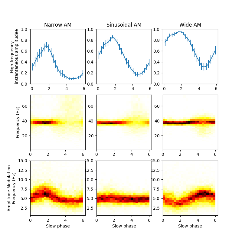
We can summarise holo_by_phase a few ways. To start we we plot the high-frequency instantaneous amplitude on the top-row for reference. The second row contains the first-layer frequencies in the Holospectrum as a function of 5Hz phase, finally the third row contains the second-layer amplitude modulation frequencies across 5Hz phase.

plt.figure(figsize=(8, 8))
plt.subplot(331)
plt.errorbar(phase_bins, ia_by_phase_narrow, yerr=ia_by_phase_narrow_var)
plt.ylim(0, 1)
plt.ylabel('High-frequency\ninstantaneous amplitudee')
plt.title('Narrow AM')
plt.subplot(332)
plt.errorbar(phase_bins, ia_by_phase, yerr=ia_by_phase_var)
plt.ylim(0, 1)
plt.title('Sinusoidal AM')
plt.subplot(333)
plt.errorbar(phase_bins, ia_by_phase_wide, yerr=ia_by_phase_wide_var)
plt.ylim(0, 1)
plt.title('Wide AM')

plt.subplot(334)
plt.pcolormesh(phase_centres, freq_centres, holo_by_phase_narrow.sum(axis=1).T,  cmap='hot_r', shading='auto')
plt.ylabel('Frequency (Hz)')
plt.subplot(335)
plt.pcolormesh(phase_centres, freq_centres, holo_by_phase.sum(axis=1).T, cmap='hot_r', shading='auto')
plt.subplot(336)
plt.pcolormesh(phase_centres, freq_centres, holo_by_phase_wide.sum(axis=1).T, cmap='hot_r', shading='auto')

plt.subplot(337)
plt.pcolormesh(phase_centres, freq_centres_low, holo_by_phase_narrow.sum(axis=2).T, cmap='hot_r', shading='auto')
plt.ylabel('Amplitude Modulation\nFrequency (Hz)')
plt.xlabel('Slow phase')
plt.subplot(338)
plt.pcolormesh(phase_centres, freq_centres_low, holo_by_phase.sum(axis=2).T, cmap='hot_r', shading='auto')
plt.xlabel('Slow phase')
plt.subplot(339)
plt.pcolormesh(phase_centres, freq_centres_low, holo_by_phase_wide.sum(axis=2).T, cmap='hot_r', shading='auto')
plt.xlabel('Slow phase')

Out:

Text(0.5, 58.7222222222222, 'Slow phase')

The second row here is very similar to the HHT-by-phase plot in our previous section and confirms that there is a peak in 37Hz power around pi/2 in the low-frequency phase. Again, the width of the modulation is visible as stretching of the peak in the x-axis.

The third row gives us some new information about how amplitude modulation frequency of the 37Hz frequency signal changes across the phase of the 5Hz signal. This is a flat profile at 5Hz for the sinsoidal signal but changes for the narrow and wide case. Critically the narrow amplitude modulation has an increase in amplitude modulation frequency around pi/2 - the point in the low-frequency signal where the high-frequency signal peaks. In contrast, the wide modulation signal has a lower amplitude modulation frequency at the same point. This reflects the fast-sharp peak in the narrow modualtion and the flat peak in the wide modulation.

All three signals are clearly linked to the low-frequency phase. Interestingly, the holospectrum is able to quantify the non-linear differences in amplitude modulation frequency driven by the diferences in modulation width.

previous

The Holospectrum

next

Cycle detection from IMFs