Intro to the sift

This tutorial is a general introduction to the sift algorithm. We introduce the sift in steps and some of the options that can be tuned.

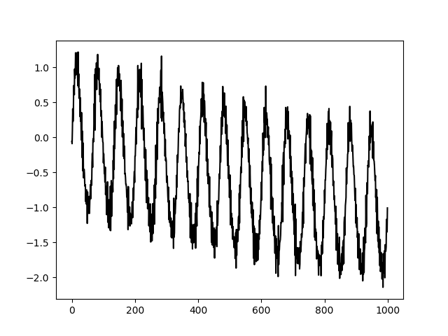
Lets make a simulated signal to get started. This is a fairly complicated signal with a non-linear 12Hz oscillation, a very slow fluctuation and some high frequency noise.

import emd
import numpy as np
from scipy import signal
import matplotlib.pyplot as plt


sample_rate = 1000
seconds = 1
num_samples = sample_rate*seconds
time_vect = np.linspace(0, seconds, num_samples)
freq = 15

# Change extent of deformation from sinusoidal shape [-1 to 1]
nonlinearity_deg = .25

# Change left-right skew of deformation [-pi to pi]
nonlinearity_phi = -np.pi/4

# Create a non-linear oscillation
x = emd.simulate.abreu2010(freq, nonlinearity_deg, nonlinearity_phi, sample_rate, seconds)

x -= np.sin(2 * np.pi * 0.22 * time_vect)   # Add part of a very slow cycle as a trend

# Add a little noise - with low frequencies removed to make this example a
# little cleaner...
np.random.seed(42)
n = np.random.randn(1000,) * .2
nf = signal.savgol_filter(n, 3, 1)
n = n - nf

x = x + n

plt.figure()
plt.plot(x, 'k')

# sphinx_gallery_thumbnail_number = 8

[<matplotlib.lines.Line2D object at 0x7f0ebb40cb50>]

The sift works by iteratively extracting oscillatory components from a signal. Starting from the fastest and through to the very slowest until only a non-oscillatory trend is left. Each component is then known as an ‘Intrinsic Mode Function’ or IMF.

The extraction of these IMFs is a difficult problem without a clear analytic or symbolic solution. Therefore, the sift looks to iteratively approximate the best set of IMFs using a set of heuristic rules (this sort of analysis is a type of numerical algorithm).

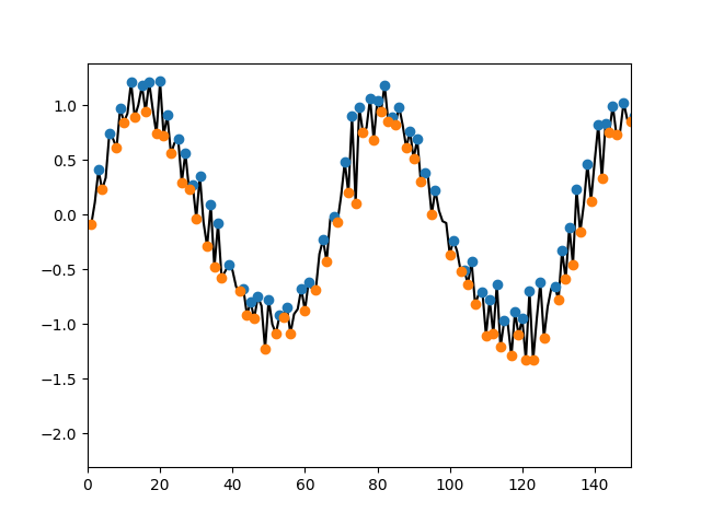
The first thing the sift does is identify the very fastest dynamics in a signal. We do this by identifying all the peaks and troughs in the signal. Here, we do this with emd.sift.get_padded_extrema and plot the extrema on a segment of the signal.

peak_locs, peak_mags = emd.sift.get_padded_extrema(x, pad_width=0, mode='peaks')
trough_locs, trough_mags = emd.sift.get_padded_extrema(x, pad_width=0, mode='troughs')

plt.figure()
plt.plot(x, 'k')
plt.plot(peak_locs, peak_mags, 'o')
plt.plot(trough_locs, trough_mags, 'o')
plt.xlim(0, 150)

(0.0, 150.0)

We want to extract the fastest dynamics from this signal - but what do we mean by fastest? We define the fastest dynamics to be the oscillations occurring between adjacent peaks and troughs in our signal - anything slower should be removed for now.

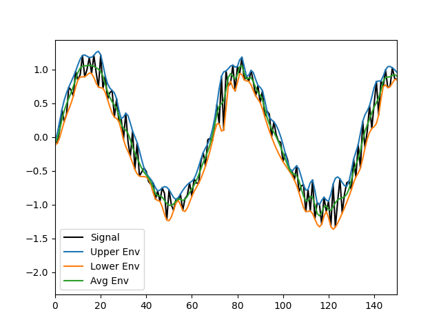
To isolate these fast dynamics, we identify an upper and lower amplitude envelope from the peaks and troughs and compute their average. Here we do this with emd.sift.interp_envelope (note: this uses emd.sift.get_padded_extrema internally to find the same extrema we plotted above) and then plot an example.

proto_imf = x.copy()
# Compute upper and lower envelopes
upper_env = emd.sift.interp_envelope(proto_imf, mode='upper')
lower_env = emd.sift.interp_envelope(proto_imf, mode='lower')

# Compute average envelope
avg_env = (upper_env+lower_env) / 2

plt.figure()
plt.plot(x, 'k')
plt.plot(upper_env)
plt.plot(lower_env)
plt.plot(avg_env)
plt.xlim(0, 150)
plt.legend(['Signal', 'Upper Env', 'Lower Env', 'Avg Env'])

<matplotlib.legend.Legend object at 0x7f0ebb406650>

In this segment, we can see that the fastest dynamics occur in the rapid oscillations of the black line between its upper a lower envelope. These oscillations are happening alongside dynamics on other time-scales which are all summed together to make the original signal. We approximate these slower dynamics through the average of the uppers and lower envelope - the green line in the plot above). The average envelope drifts more slowly than the fastest oscillations visible in the raw signal and tends to capture trends in the mean across several cycles of the fastest dynamics.

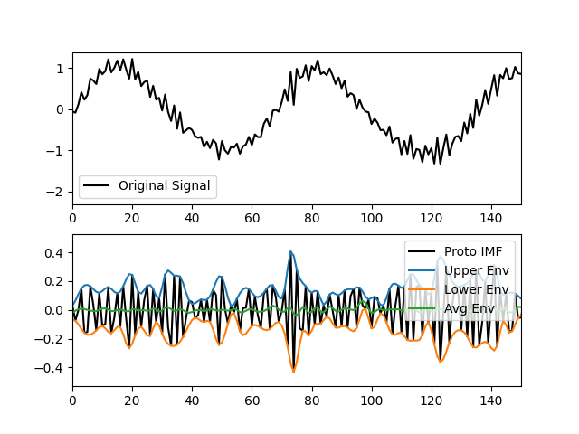
We can remove these slower components by simply subtracting this average envelope. Here we do this subtraction and make a quick plot

# Subtract slow dynamics from previous cell
proto_imf = x - avg_env

# Compute upper and lower envelopes
upper_env = emd.sift.interp_envelope(proto_imf, mode='upper')
lower_env = emd.sift.interp_envelope(proto_imf, mode='lower')

# Compute average envelope
avg_env = (upper_env+lower_env) / 2

plt.figure()
plt.subplot(211)
plt.plot(x, 'k')
plt.xlim(0, 150)
plt.legend(['Original Signal'])

plt.subplot(212)
plt.plot(proto_imf, 'k')
plt.plot(upper_env)
plt.plot(lower_env)
plt.plot(avg_env)
plt.xlim(0, 150)
plt.legend(['Proto IMF', 'Upper Env', 'Lower Env', 'Avg Env'])

<matplotlib.legend.Legend object at 0x7f0ebb59d490>

The top panel shows the original signal and average envelope, and the bottom panel shows the signal with the average envelope removed and the envelopes of this new signal.

The fastest oscillations are now much clearer with the slow trends removed. The sift algorithm now just repeats these steps until certain stopping conditions are met. In general, we want to stop sifting an IMF once the average of the upper and lower envelopes are sufficiently close to zero. When this condition is met, it guarantees that the signal will behave well during analysis of instantaneous frequency (a story for another tutorial…).

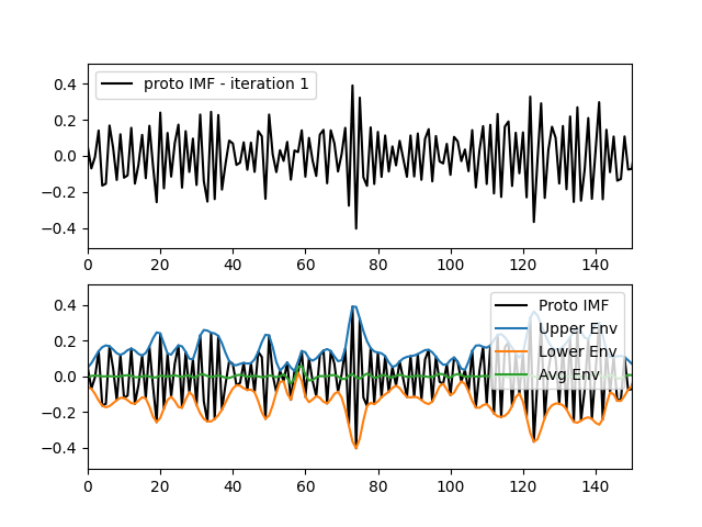
Here we run another iteration of the sift on the residual of our previous one.

# Subtract slow dynamics from previous cell
proto_imf = proto_imf - avg_env

# Compute upper and lower envelopes
upper_env = emd.sift.interp_envelope(proto_imf, mode='upper')
lower_env = emd.sift.interp_envelope(proto_imf, mode='lower')

# Compute average envelope
avg_env = (upper_env+lower_env) / 2

plt.figure()
plt.subplot(211)
plt.plot(proto_imf, 'k')
plt.xlim(0, 150)
plt.legend(['proto IMF - iteration 1'])

plt.subplot(212)
plt.plot(proto_imf, 'k')
plt.plot(upper_env)
plt.plot(lower_env)
plt.plot(avg_env)
plt.xlim(0, 150)
plt.legend(['Proto IMF', 'Upper Env', 'Lower Env', 'Avg Env'])

<matplotlib.legend.Legend object at 0x7f0ebb618a10>

After two iterations the average envelope is now very closer to zero though there are still some deviations. The full sift would continue iterating until we pass a defined threshold and accept the result as our IMF.

Running sift iterations

We don’t want to run these iterations by hand, so lets define a function to do the work for us. Here, we make my_get_next_imf which will repeat the steps above until the average envelopes are sufficiently close to zero as defined by the sd_thresh. We will plot the sift ierations as we go and include an option to zoom in in part of the signal.

def my_get_next_imf(x, zoom=None, sd_thresh=0.1):

    proto_imf = x.copy()  # Take a copy of the input so we don't overwrite anything
    continue_sift = True  # Define a flag indicating whether we should continue sifting
    niters = 0            # An iteration counter

    if zoom is None:
        zoom = (0, x.shape[0])

    # Main loop - we don't know how many iterations we'll need so we use a ``while`` loop
    while continue_sift:
        niters += 1  # Increment the counter

        # Compute upper and lower envelopes
        upper_env = emd.sift.interp_envelope(proto_imf, mode='upper')
        lower_env = emd.sift.interp_envelope(proto_imf, mode='lower')

        # Compute average envelope
        avg_env = (upper_env+lower_env) / 2

        # Add a summary subplot
        plt.subplot(5, 1, niters)
        plt.plot(proto_imf[zoom[0]:zoom[1]], 'k')
        plt.plot(upper_env[zoom[0]:zoom[1]])
        plt.plot(lower_env[zoom[0]:zoom[1]])
        plt.plot(avg_env[zoom[0]:zoom[1]])

        # Should we stop sifting?
        stop, val = emd.sift.stop_imf_sd(proto_imf-avg_env, proto_imf, sd=sd_thresh)

        # Remove envelope from proto IMF
        proto_imf = proto_imf - avg_env

        # and finally, stop if we're stopping
        if stop:
            continue_sift = False

    # Return extracted IMF
    return proto_imf

The core parts of this function should be familiar from earlier parts of the tutorial. We can now call this function to find the fastest IMF from our signal.

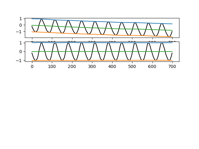
Let’s extract our IMF, plotting the iterations and zooming in to a 100 sample period so we can see the details.

imf1 = my_get_next_imf(x, zoom=(100, 200))

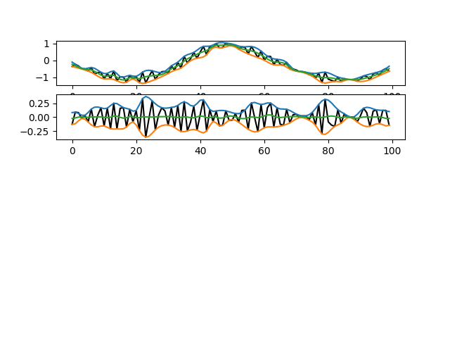
The top panel shows the original signal and each lower panel shows successive iterations. The first iteration removes the majority of the slow oscillation whilst the second does some fine-tuning.

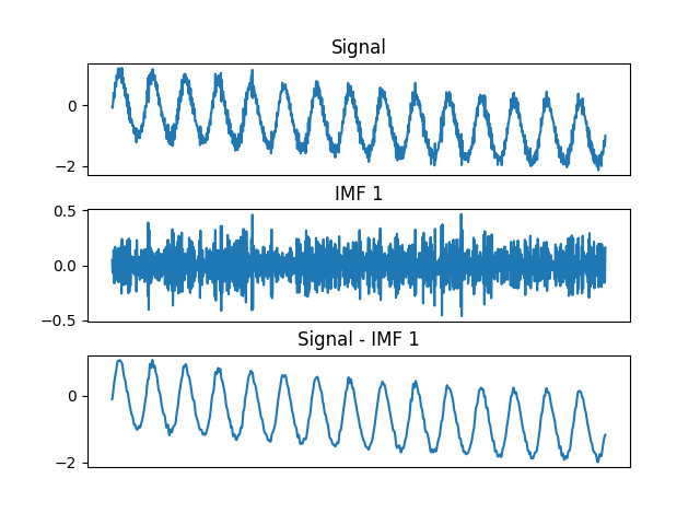
Here we plot the original signal, the first IMF and the residual after subtracting the first IMF from the signal.

plt.figure()
plt.subplots_adjust(hspace=0.3)

plt.subplot(311)
plt.plot(x)
plt.title('Signal')
plt.xticks([])

plt.subplot(312)
plt.plot(imf1)
plt.title('IMF 1')
plt.xticks([])

plt.subplot(313)
plt.plot(x - imf1)
plt.title('Signal - IMF 1')
plt.xticks([])

([], [])

There are some edge effects visible in our IMF. This is due to uncertainty in the envelope interpolation at the edges of the signal. The residual of the signal minus the IMF now has a lot of high frequency content removed.

We can repeat the process on this residual to identify our next IMF. The process of peak detection, envelope interpolation and subtraction is identical for this second IMF. Critically, as we’ve removed the first IMF - the peaks will be further apart in this iteration and we will extract slower dynamics. Therefore we zoom into a slightly longer 200 sample window.

imf2 = my_get_next_imf(x - imf1, zoom=(100, 300))

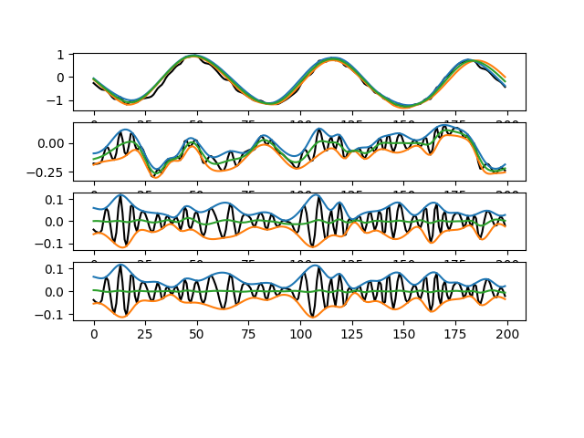
This IMF is tiny! The first couple of iterations remove the big slow oscillations and after four iterations we have a very small amplitude component containing a clean oscillation with zero mean.

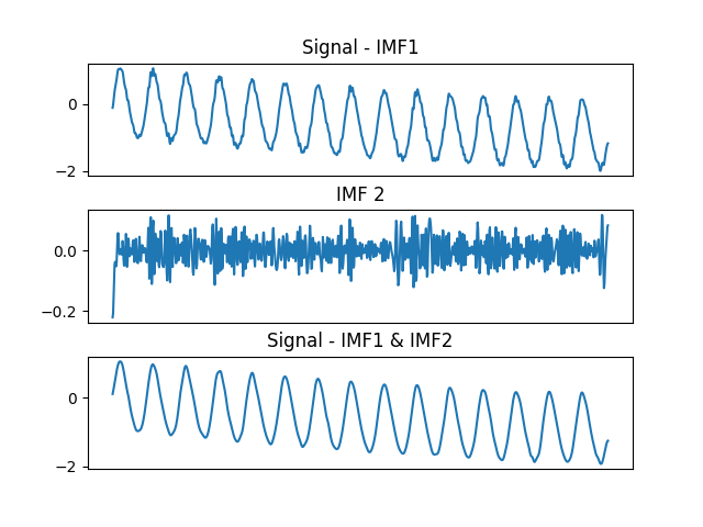
After subtracting both IMFs the larger 12 Hz oscillation now looks very smooth.

plt.figure()
plt.subplots_adjust(hspace=0.3)

plt.subplot(311)
plt.plot(x - imf1)
plt.title('Signal - IMF1')
plt.xticks([])

plt.subplot(312)
plt.plot(imf2)
plt.title('IMF 2')
plt.xticks([])

plt.subplot(313)
plt.plot(x - imf1 - imf2)
plt.title('Signal - IMF1 & IMF2')
plt.xticks([])

([], [])

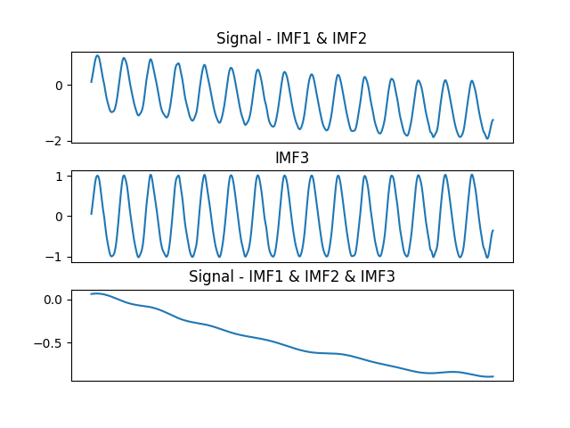
The next IMF extraction is very simple. It only takes a single iteration to remove the slow drift from the 12Hz oscillation

imf3 = my_get_next_imf(x - imf1 - imf2, zoom=(100, 800))

The residual of the signal with the first 3 IMFs is now close to a trend.

plt.figure()
plt.subplots_adjust(hspace=0.3)

plt.subplot(311)
plt.plot(x - imf1 - imf2)
plt.title('Signal - IMF1 & IMF2')
plt.xticks([])

plt.subplot(312)
plt.plot(imf3)
plt.title('IMF3')
plt.xticks([])

plt.subplot(313)
plt.plot(x - imf1 - imf2 - imf3)
plt.title('Signal - IMF1 & IMF2 & IMF3')
plt.xticks([])

([], [])

The top-level sift function

This whole process is implemented in emd.sift.sift. Here we run the sift using the top level function and recover the same components as we generated during this tutorial.

imf = emd.sift.sift(x, imf_opts={'sd_thresh': 0.1})
emd.plotting.plot_imfs(imf)

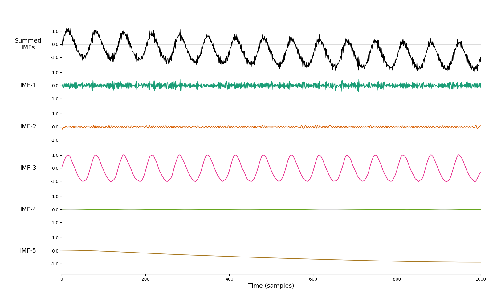
<Axes: xlabel='Time (samples)'>

emd.sift.sift is highly customisable with many options tuning the peak detection, envelope interpolation and sift thresholds.

Further Reading & References

Huang, N. E., Shen, Z., Long, S. R., Wu, M. C., Shih, H. H., Zheng, Q., … Liu, H. H. (1998). The empirical mode decomposition and the Hilbert spectrum for nonlinear and non-stationary time series analysis. Proceedings of the Royal Society of London. Series A: Mathematical, Physical and Engineering Sciences, 454(1971), 903–995. https://doi.org/10.1098/rspa.1998.0193