Note
Go to the end to download the full example code.
The sift in detail#
Here, we will run through the different steps of the sift and get to know some of the lower-level functions which are used by the core sift functions. There are four levels of functions which are used in the sift.
We will take a look at each of these steps in turn using a simulated time-series.
Lets make a simulated signal to get started.
import emd
import numpy as np
import matplotlib.pyplot as plt

sample_rate = 1000
seconds = 10
num_samples = sample_rate*seconds
time_vect = np.linspace(0, seconds, num_samples)
freq = 5

# Change extent of deformation from sinusoidal shape [-1 to 1]
nonlinearity_deg = .25

# Change left-right skew of deformation [-pi to pi]
nonlinearity_phi = -np.pi/4

# Create a non-linear oscillation
x = emd.simulate.abreu2010(freq, nonlinearity_deg, nonlinearity_phi, sample_rate, seconds)

x += np.cos(2 * np.pi * 1 * time_vect)        # Add a simple 1Hz sinusoid
x -= np.sin(2 * np.pi * 2.2e-1 * time_vect)   # Add a very slow cycle

# sphinx_gallery_thumbnail_number = 7
Sifting#
The top-level of options configure the sift itself. These options vary between the type of sift that is being performed and options don’t generalise between different variants of the sift.
Here we will run a standard sift on our simulation.
# Get the default configuration for a sift
config = emd.sift.get_config('sift')
# Adjust the threshold for accepting an IMF
config['imf_opts/sd_thresh'] = 0.05
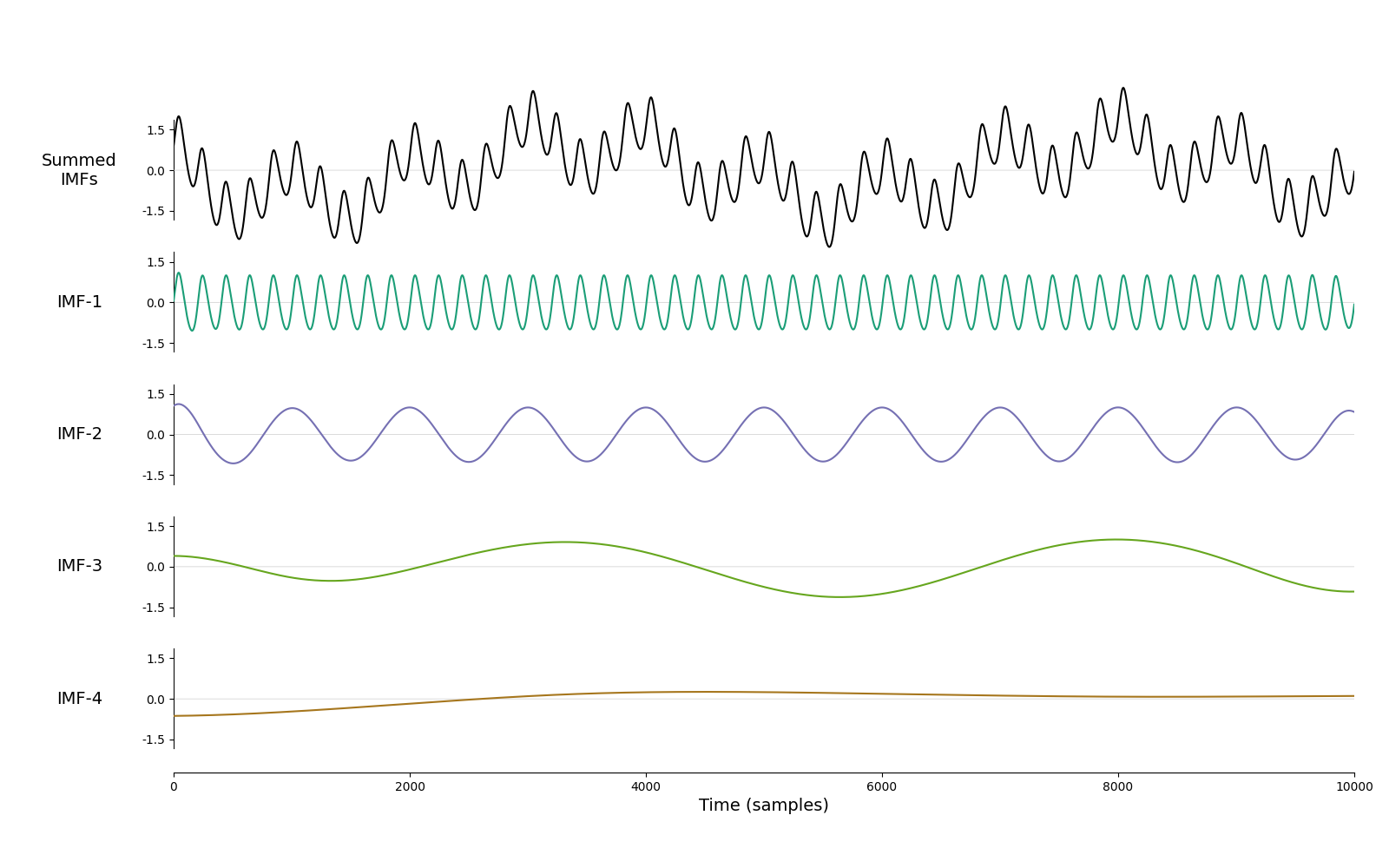
imf = emd.sift.sift(x)
emd.plotting.plot_imfs(imf)

<Axes: xlabel='Time (samples)'>
# Get the default configuration for a sift
config = emd.sift.get_config('sift')
# Adjust the threshold for accepting an IMF
config['imf_opts/sd_thresh'] = 0.05
config['extrema_opts/method'] = 'rilling'

imf = emd.sift.sift(x)

emd.plotting.plot_imfs(imf)

<Axes: xlabel='Time (samples)'>
- Internally the
siftfunction calls a set of lower level functions to extract the IMFs. These functions are call in a hierarchy when you run
siftit will callget_next_imfbehind the scenes. Similarly,get_next_imfmakes use ofinterp_envelopeand so on.
get_next_imfextracts the fastest IMF from an input signalinterp_envelopefind the interpolated envelope of a signal.get_padded_extremaidentifies the location and magnitude of signal extrema with optional padding.
We will run through each of these functions in now, giving some examples of their use and options.
IMF Extraction#
After the top-level sift function, the next layer is IMF extraction as
implemented in emd.sift.get_next_imf. This uses the envelope
interpolation and extrema detection to carry out the sifting iterations on a
time-series to return a single intrinsic mode function.
This is the main function used when implementing novel types of sift. For
instance, the ensemble sift uses this emd.sift.get_next_imf to extract
IMFs from many repetitions of the signal with small amounts of noise added.
Similarly the mask sift calls emd.sift.get_next_imf after adding a mask
signal to the data.
Here we call get_next_imf repeatedly on a signal and its residuals to
implement a very simple sift. We extract the first IMF, subtract it from the
data and then extract the second and third IMFs. We then plot the original
signal, the IMFs and the residual.
# Extract the options for get_next_imf - these can be customised here at this point.
imf_opts = config['imf_opts']

# Extract first IMF from the signal
imf1, continue_sift = emd.sift.get_next_imf(x[:, None],           **imf_opts)

# Extract second IMF from the signal with the first IMF removed
imf2, continue_sift = emd.sift.get_next_imf(x[:, None]-imf1,      **imf_opts)

# Extract third IMF from the signal with the first and second IMFs removed
imf3, continue_sift = emd.sift.get_next_imf(x[:, None]-imf1-imf2, **imf_opts)

# The residual is the signal component left after removing the IMFs
residual = x[:, None] - imf1 - imf2 - imf3

# Contactenate our IMFs into one array
imfs_manual = np.c_[imf1, imf2, imf3, residual]

# Visualise
emd.plotting.plot_imfs(imfs_manual)
<Axes: xlabel='Time (samples)'>
These IMFs should be identical to the IMFs obtained using emd.sift.sift above.
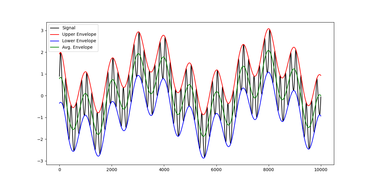
Envelope interpolation#
A large part of IMF exraction is the computation of an upper and lower
envelope of the signal. This is done through interpolation using
emd.sift.interp_envelope and the options in the envelope section of
the config.
# Extract envelope options
env_opts = config['envelope_opts']

# Compute upper and lower envelopes
upper_env = emd.sift.interp_envelope(x, mode='upper', **env_opts)
lower_env = emd.sift.interp_envelope(x, mode='lower', **env_opts)

# Compute average envelope
avg_env = (upper_env+lower_env) / 2

# Visualise
plt.figure(figsize=(12, 6))
plt.plot(x, 'k')
plt.plot(upper_env, 'r')
plt.plot(lower_env, 'b')
plt.plot(avg_env, 'g')
plt.legend(['Signal', 'Upper Envelope', 'Lower Envelope', 'Avg. Envelope'])
<matplotlib.legend.Legend object at 0x7cd7a6f34750>
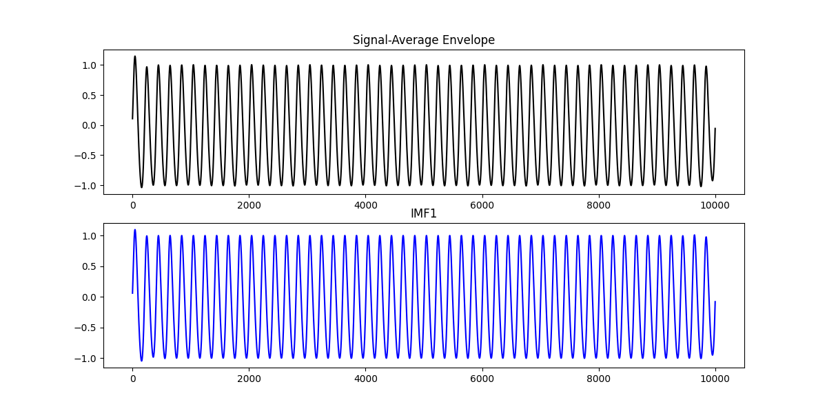
Subtracting the upper and lower envelopes from the signal removes slow dynamics from the signal. Next, we subtract the average envelope from our signal.
# Plot the signal with the average of the upper and lower envelopes subtracted alongside IMF1
plt.figure(figsize=(12, 6))
plt.subplot(211)
plt.plot(x-avg_env, 'k')
plt.title('Signal-Average Envelope')
plt.subplot(212)
plt.plot(imf1, 'b')
plt.title('IMF1')
Text(0.5, 1.0, 'IMF1')
Note that the simple subtraction is very similar to IMF1 as extracted above. In real data, several iterations of envelope computation and subtraction may be required to identify a well-formed IMF.
In this case there is a small amplitude error in the IMF at the very start. This is due to uncertainty in the envelope interpolation at the edges. This can sometimes be reduced by changing the interpolation and extrema padding options but is hard to completely overcome. It is often sensible to treat the first and last couple of cycles in an IMF with caution.
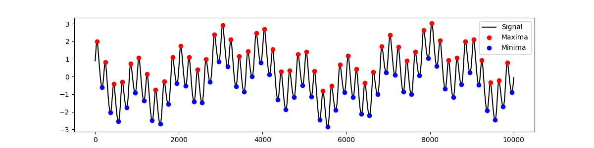
Extrema detection and padding#
Finally, the lowest-level functions involve extrema detection and padding as
implemented in the emd.sift.get_padded_extrema function. This is a simple
function which identifies extrema using scipy.signal. Here we identify
peaks and troughs without any padding applied.
max_locs, max_mag = emd.sift.get_padded_extrema(x, pad_width=0, mode='peaks')
min_locs, min_mag = emd.sift.get_padded_extrema(x, pad_width=0, mode='troughs')

plt.figure(figsize=(12, 3))
plt.plot(x, 'k')
plt.plot(max_locs, max_mag, 'or')
plt.plot(min_locs, min_mag, 'ob')
plt.legend(['Signal', 'Maxima', 'Minima'])
<matplotlib.legend.Legend object at 0x7cd7ac0ba310>
Extrema padding is used to stablise the envelope at the edges of the
time-series. The emd.sift.get_padded_extrema function identifies and pads
extrema in a time-series. This calls the emd.sift.find_extrema internally.
plt.figure(figsize=(12, 7))

# Method 1 - np.pad
max_locs, max_mag = emd.sift.get_padded_extrema(x, pad_width=2, mode='peaks', method='numpypad')
min_locs, min_mag = emd.sift.get_padded_extrema(x, pad_width=2, mode='troughs', method='numpypad')

plt.subplot(211)
plt.plot(x, 'k')
plt.plot(max_locs, max_mag, 'or')
plt.plot(min_locs, min_mag, 'ob')
plt.legend(['Signal', 'Maxima', 'Minima'])
plt.title('default numpy.pad method')

# Method 2 - Rillings method
max_locs, max_mag = emd.sift.get_padded_extrema(x, pad_width=4, mode='peaks', method='rilling')
min_locs, min_mag = emd.sift.get_padded_extrema(x, pad_width=4, mode='troughs', method='rilling')

plt.subplot(212)
plt.plot(x, 'k')
plt.plot(max_locs, max_mag, 'or')
plt.plot(min_locs, min_mag, 'ob')
plt.legend(['Signal', 'Maxima', 'Minima'])
plt.title('Rillings Method')
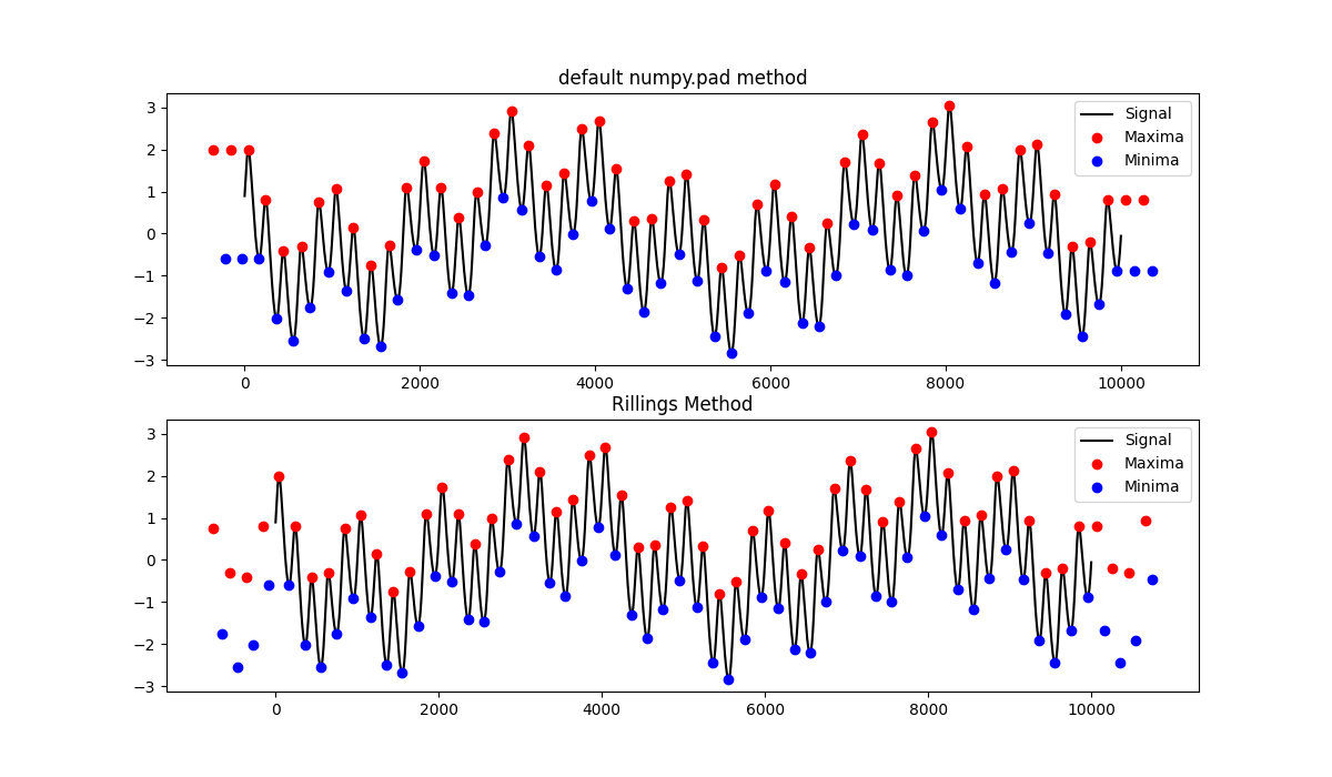
Text(0.5, 1.0, 'Rillings Method')
Extrema padding is used to stablise the envelope at the edges of the
time-series. The emd.sift.get_padded_extrema function identifies and pads
extrema in a time-series. This calls the emd.sift.find_extrema internally.
plt.figure(figsize=(12, 7))

env, extr = emd.sift.interp_envelope(x, ret_extrema=True, extrema_opts={'method': 'numpypad'}, trim=False)
plt.subplot(211)
plt.plot(x, 'k')
plt.plot(extr[0], extr[1], 'or')
plt.plot(extr[2], extr[3], 'ob')
plt.plot(np.arange(extr[0][0], extr[0][-1]), env[1])
plt.plot(np.arange(extr[2][0], extr[2][-1]), env[0])
plt.legend(['Signal', 'Maxima', 'Minima', 'Upper Env', 'Lower Env'])
plt.title('np.pad Method')

env, extr = emd.sift.interp_envelope(x, ret_extrema=True, extrema_opts={'method': 'rilling'}, trim=False)
plt.subplot(212)
plt.plot(x, 'k')
plt.plot(extr[0], extr[1], 'or')
plt.plot(extr[2], extr[3], 'ob')
plt.plot(np.arange(extr[0][0], extr[0][-1]), env[1])
plt.plot(np.arange(extr[2][0], extr[2][-1]), env[0])
plt.legend(['Signal', 'Maxima', 'Minima', 'Upper Env', 'Lower Env'])
plt.title('Rillings Method')
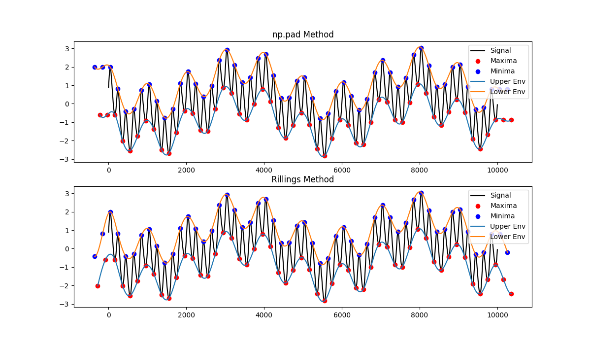
Text(0.5, 1.0, 'Rillings Method')
The extrema detection and padding arguments are specified in the config dict
under the extrema, mag_pad and loc_pad keywords. These are passed directly
into emd.sift.get_padded_extrema when running the sift.
The default extrema padding uses Rilling’s method, but we can switch this to
use a built in numpy function np.pad. The mag_pad and loc_pad
dictionaries are passed into np.pad to define the padding in the y-axis
(extrema magnitude) and x-axis (extrema time-point) respectively. Note that
np.pad takes a mode as a positional argument - this must be included as a
keyword argument here.
Lets try customising the extrema padding. First we get the ‘extrema’ options from a nested config then try changing a couple of options
ext_opts = config['extrema_opts']
ext_opts['method'] = 'numpypad'

# The default options
max_locs, max_mag = emd.sift.get_padded_extrema(x, mode='peaks', **ext_opts)
min_locs, min_mag = emd.sift.get_padded_extrema(x, mode='troughs', **ext_opts)

plt.figure(figsize=(12, 12))

plt.subplot(311)
plt.plot(x, 'k')
plt.plot(max_locs, max_mag, 'or')
plt.plot(min_locs, min_mag, 'ob')
plt.legend(['Signal', 'Maxima', 'Minima'])
plt.title('Default')

# Increase the pad width to 5 extrema
ext_opts['pad_width'] = 5
max_locs, max_mag = emd.sift.get_padded_extrema(x, mode='peaks', **ext_opts)
min_locs, min_mag = emd.sift.get_padded_extrema(x, mode='troughs', **ext_opts)

plt.subplot(312)
plt.plot(x, 'k')
plt.plot(max_locs, max_mag, 'or')
plt.plot(min_locs, min_mag, 'ob')
plt.legend(['Signal', 'Maxima', 'Minima'])
plt.title('Increased pad width')

# Change the y-axis padding to 'reflect' rather than 'median' (this option is
# for illustration and not recommended for actual sifting....)
ext_opts['mag_pad_opts']['mode'] = 'reflect'
del ext_opts['mag_pad_opts']['stat_length']
max_locs, max_mag = emd.sift.get_padded_extrema(x, mode='peaks', **ext_opts)
min_locs, min_mag = emd.sift.get_padded_extrema(x, mode='troughs', **ext_opts)

plt.subplot(313)
plt.plot(x, 'k')
plt.plot(max_locs, max_mag, 'or')
plt.plot(min_locs, min_mag, 'ob')
plt.legend(['Signal', 'Maxima', 'Minima'])
plt.title('Reflected extrema and increased pad width')
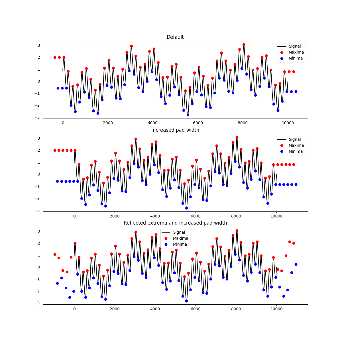
Text(0.5, 1.0, 'Reflected extrema and increased pad width')
Further Reading & References#
Huang, N. E., Shen, Z., Long, S. R., Wu, M. C., Shih, H. H., Zheng, Q., … Liu, H. H. (1998). The empirical mode decomposition and the Hilbert spectrum for nonlinear and non-stationary time series analysis. Proceedings of the Royal Society of London. Series A: Mathematical, Physical and Engineering Sciences, 454(1971), 903–995. https://doi.org/10.1098/rspa.1998.0193
Total running time of the script: (0 minutes 1.270 seconds)